Analyzing AutoStructure Output Directories: Difference between revisions
No edit summary |
No edit summary |
||
| (4 intermediate revisions by 2 users not shown) | |||
| Line 1: | Line 1: | ||
== '''Introduction''' == | == '''Introduction''' == | ||
In this section we describe how to analyze AutoStructure results using the graphical user interface (GUI). | In this section we describe how to analyze AutoStructure version 2.2.1 results using the graphical user interface (GUI). | ||
== '''Methods''' == | == '''Methods''' == | ||
| Line 9: | Line 9: | ||
=== AutoStructure Directory Tree === | === AutoStructure Directory Tree === | ||
The results of each AutoStructure cycle are nicely collected in directories within the parent output directory specified by the user in the structure calculation command by clicking the Tree View tab (see Figure 1). | The results of each AutoStructure cycle are nicely collected in directories within the parent output directory specified by the user in the structure calculation command by clicking the Tree View tab (see Figure 1). Clicking any of the files opens up their contents in another window. | ||
==== Figure 1: AutoStructure Directory Tree ==== | ==== Figure 1: AutoStructure Directory Tree ==== | ||
[[Image:ASoutput tree.png]] | [[Image:ASoutput tree.png|528x561px]] | ||
<br> | <br> | ||
| Line 44: | Line 44: | ||
==== Figure 2: AutoStructure Summary Page ==== | ==== Figure 2: AutoStructure Summary Page ==== | ||
[[Image:ASoutput fig1.png]] | [[Image:ASoutput fig1.png|563x732px]] | ||
The user can click any cycle box near the botton of the page and obtain a summary of the backbone, sidechain, intraresidue, medium and long range NOE assignments made in that cycle for that peak list (Figure 3). | The user can click any cycle box near the botton of the page and obtain a summary of the backbone, sidechain, intraresidue, medium and long range NOE assignments made in that cycle for that peak list (Figure 3). | ||
| Line 50: | Line 50: | ||
==== Figure 3: Peak List Assignment Information for a Cycle ==== | ==== Figure 3: Peak List Assignment Information for a Cycle ==== | ||
[[Image:ASoutput fig1b.png]] | [[Image:ASoutput fig1b.png|544x397px]] | ||
=== Initial Fold Analysis === | === Initial Fold Analysis === | ||
| Line 58: | Line 58: | ||
==== Figure 4: Initial Fold Analysis ==== | ==== Figure 4: Initial Fold Analysis ==== | ||
[[Image:ASoutput initialfold.png| | [[Image:ASoutput initialfold.png|694x532px]] | ||
=== Contact Map Display === | |||
The Contact Maps tab provides, for each cycle, grid maps of all interactions between pairs of residues (Figure 5). Backbone interactions are shown in red in the lower portion of the plot and backbone + side chain interactions are shown in the top half of the plot. The user can click on any point in the map and open a box containing all NOE contact information between those residues, and the user can subsequently view the exact peaks which contribute to this point in the map. This tool is especially useful for finding potentially spurious peaks, which would manifest as outliers in this plot, and not supported by any other peak in the assignment. | |||
==== Figure 5: An AutoStructure Contact Map ==== | |||
[[Image:ASoutput contact.png|647x684px]] | |||
=== Checklist === | |||
The Checklist tab provides the user a list of all unassigned peaks in the final structure, which were assigned at some intermediate step in the run. Each peak is displayed along with the peak list, cycle it would unassigned, and rational for why it was assigned and then unassigned. Again, this is a useful tool for eliminating potential spurious peaks or for identifying chemical shift assignment errors. | |||
=== NOE Assignments === | |||
The NOE Assignments tab provides complete assignment lists for each peak lists used in the calculation. The output is in the format and exact order of peaks provided by the user. Unassigned peaks are also shown. The user can click on any peak and produce a box with all possible residue assignments for that peak, distances in the final structure, and rationale for assigning/unassigning that peak. | |||
<br> | |||
<br> | |||
Latest revision as of 21:35, 6 January 2010
Introduction
In this section we describe how to analyze AutoStructure version 2.2.1 results using the graphical user interface (GUI).
Methods
One can access the entire output directory using the AutoStructrue GUI, under the AutoStructure pull-down menu -> Open AS OuputDir.
AutoStructure Directory Tree
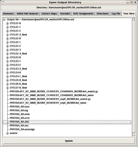
The results of each AutoStructure cycle are nicely collected in directories within the parent output directory specified by the user in the structure calculation command by clicking the Tree View tab (see Figure 1). Clicking any of the files opens up their contents in another window.
Figure 1: AutoStructure Directory Tree
Here is a description of the files collected in the output directory:
- CYCLE directories:
- CYCLE1-0: initial fold analysis results
- CYCLE*-0: iterative fold analysis
- others: validation cycles
- each CYCLE directory contains:
- log files for all the calculations run
- the parameter and constraint files used in the structure calculations for that run
- assigned NOESY peak lists that can be read back into Sparky.
- filename_NA.ovw: general report on the AuotStructure calculation, including M-scores and global referencing for each NOESY peak list, and the final statistics for each cycle in the run
- filename_NA.sec: secondary structure analysis
- filename_NA.exm: complete secondary initial fold analysis report
- filename_NA.unassign: list of unsassigned peaks during each cycle of the run
- filename_NA.note: report on the preprocessing of the input files and errors
- filename_NA.QM: summary of M scores. It provides guidance for chemical shift assignment and peak picking
- filename_NA.log: log file for the run
- peaklist.noise: list of peaks excluded from NOESY analysis because they do not match any chemical shift assignments (within given tolerances)
- peaklist.match: matching results for all peaks in the NOESY list
- source directory: contains the exact files used to initiate the AutoStructure run
AutoStructure Summary Page
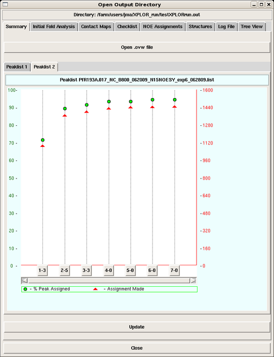
When the output directory is launched, the first view is the Summary Page, which provides plots of the total NOE assignments and percentage NOE assignments for each peak list in each cycle of the run (Figure 2).
Figure 2: AutoStructure Summary Page
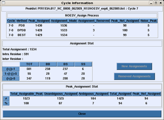
The user can click any cycle box near the botton of the page and obtain a summary of the backbone, sidechain, intraresidue, medium and long range NOE assignments made in that cycle for that peak list (Figure 3).
Figure 3: Peak List Assignment Information for a Cycle
Initial Fold Analysis
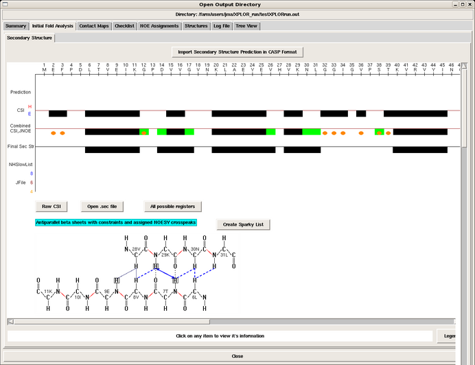
Clicking the Initial Fold Analysis tab produces a window containing the secondary structure analysis performed by AutoStructure in the initial stage of the run, given in the .sec file. Data for the analysis include: Chemical Shift Indexing (CSI), scalar coupling data, slow NH exchange data, and NOE information. All of this information is mapped onto the sequence. The program also displays the possible antiparallel and parallel beta strand registers in the protein, with supporting NOE interactions shown in blue (Figure 4).
Figure 4: Initial Fold Analysis
Contact Map Display
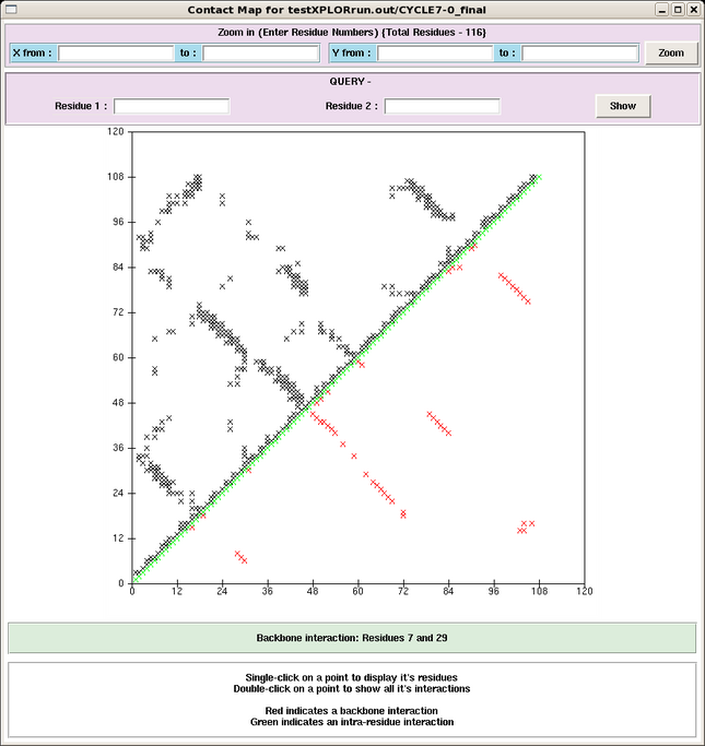
The Contact Maps tab provides, for each cycle, grid maps of all interactions between pairs of residues (Figure 5). Backbone interactions are shown in red in the lower portion of the plot and backbone + side chain interactions are shown in the top half of the plot. The user can click on any point in the map and open a box containing all NOE contact information between those residues, and the user can subsequently view the exact peaks which contribute to this point in the map. This tool is especially useful for finding potentially spurious peaks, which would manifest as outliers in this plot, and not supported by any other peak in the assignment.
Figure 5: An AutoStructure Contact Map
Checklist
The Checklist tab provides the user a list of all unassigned peaks in the final structure, which were assigned at some intermediate step in the run. Each peak is displayed along with the peak list, cycle it would unassigned, and rational for why it was assigned and then unassigned. Again, this is a useful tool for eliminating potential spurious peaks or for identifying chemical shift assignment errors.
NOE Assignments
The NOE Assignments tab provides complete assignment lists for each peak lists used in the calculation. The output is in the format and exact order of peaks provided by the user. Unassigned peaks are also shown. The user can click on any peak and produce a box with all possible residue assignments for that peak, distances in the final structure, and rationale for assigning/unassigning that peak.
