Routine 2D Experiment: Difference between revisions
No edit summary |
No edit summary |
||
| (10 intermediate revisions by the same user not shown) | |||
| Line 5: | Line 5: | ||
===== '''Brief Description''' ===== | ===== '''Brief Description''' ===== | ||
NMRPipe is designed for multidimensional NMR processing. The preferred method of processing data is to compile the commands and functions into a script file. The script file can be easily modified for different type of experiments and | NMRPipe is designed for multidimensional NMR processing. The preferred method of processing data is to compile the commands and functions into a script file. The script file can be easily modified for different type of experiments and serves as a record of how the data was processed. An example of converting the 2D HSQC spectrometer data to NMRPipe format is shown along with processing and visualizing of the dataset. | ||
<br> | <br> | ||
===== '''Software Information''' ===== | ===== '''Software Information''' ===== | ||
| Line 43: | Line 43: | ||
===== '''Converting Spectrometer Data into NMRPipe Format''' ===== | ===== '''Converting Spectrometer Data into NMRPipe Format''' ===== | ||
To convert data from spectrometer format to NMRPipe format is usually done using the build-in program called ‘varian’ for Varian dataset (bruker for Bruker dataset and delta for dataset from JEOL). Brief summaries of the build-in | To convert data from spectrometer format to NMRPipe format is usually done using the build-in program called ‘varian’ for a Varian dataset ('bruker' for a Bruker dataset and 'delta' for dataset from JEOL). [[Brief_description_of_philosophy,_commands,_and_functions_of_NMRPipe|Brief summaries of the build-in programs can be found here.]] | ||
<br> | <br> | ||
| Line 51: | Line 51: | ||
<br> | <br> | ||
[[Image:Varian-utility-raw.png]] [[Image:Varian- | [[Image:Varian-utility-raw.png]] [[Image:Varian-script-raw.png]] | ||
<br> | <br> | ||
| Line 57: | Line 57: | ||
Step 2: Click on the ‘Read Parameters’ button and the script will read the parameter file (‘procpar’) and update the parameters. | Step 2: Click on the ‘Read Parameters’ button and the script will read the parameter file (‘procpar’) and update the parameters. | ||
<br> | <br> [[Image:Varian-utility-readed.png]] [[Image:Varian-script-readed.png]] <br> | ||
[[Image:Varian-utility-readed.png]] [[Image:Varian-script-readed.png]] | |||
<br> | |||
<br> | <br> | ||
The template shows parameters for two dimensions x and y. The x dimension is the direct dimension and is always collected as complex data (quadrature detection) and the xMODE is set as complex. The xN (real+imaginary points) parameter is twice the xT (complex points) parameter. For the indirect dimension y, the yN parameter is twice the yT parameter (number of | The template shows parameters for two dimensions x and y. The x dimension is the direct dimension and is always collected as complex data (quadrature detection) and the xMODE is set as complex. The xN (real+imaginary points) parameter is twice the xT (complex points) parameter. For the indirect dimension y, the yN parameter is twice the yT parameter (number of increments, ni for a Varian instrument)<span style="font: 12.0px Times New Roman">,</span> indicating that we are collecting complex dataset to account for ‘quadrature’ in the indirect dimension. For the sensitivity-enhanced experiments the yMODE will be set to “Rance-Kay”. The frequency values can be modified using the pull down tab. The center position ppm of each dimension (xCAR and yCAR) can be updated at this stage and it can also be update later. | ||
<br> | <br> | ||
| Line 77: | Line 75: | ||
<br> | <br> | ||
[[Image:NMRPipe-Macro-Editors.png|900px|Left]] | |||
<br> | <br> | ||
An alternative way to create | An alternative way to create a processing script is to copy an existing one and edit it with a text editor. An example of processing script for a 2D <sup>15</sup>N HSQC spectrum is shown below. The script starts off by reading in the time domain data ‘test.fid’ using the ‘nmrPipe –in’ command following by ‘\’ at the end of each line. Each subsequent ‘nmrPipe –fn’ command line will begin with a unix ‘|’ and end with ‘\’. A solvent suppression filter SOL was first applied to removed residual solvent followed by a 90 degrees sine bell squared apodization (equivalent to cosine) with scale factor for first point as 0.5. The data is then zero<span style="font: 12.0px Times New Roman">-</span>filled to the nearest power of 2, Fourier transformed, phased, and the amide region of the spectrum (left half) extracted. The TP functions transpose the data to the y-axis to apply linear prediction, apodization, zero fill, Fourier transform, phasing to the y-dimension, and output the finished file as ‘test.ft2’. When the first point is collected at a half dwell time (for a Varian instrument, f1180=’y’), the phasing values in the indirect dimension are set to ‘-90 for p0 and 180 for p1’ and the first point multiplier set to 1.0<span style="font: 12.0px Times New Roman">.</span> | ||
<br> | <br> | ||
<pre>|nmrPipe -in test.fid \ | |||
| nmrPipe -fn SOL \ ## Solvent suppresion | |||
| nmrPipe -fn SP -off 0.5 -end 1.00 -pow 2 -c 0.5 \ ## Apodization | |||
| nmrPipe -fn ZF -auto \ ## Zero fill | |||
| nmrPipe -fn FT -auto \ ## Fourier transformation | |||
| nmrPipe -fn PS -p0 13.6 -p1 0.0 -di \ ## Phase correction | |||
| nmrPipe -fn EXT –left –sw \ # Extract spectrum | |||
| nmrPipe -fn TP \ ## Transpose to the y-axis | |||
| nmrPipe -fn LP -fb \ ## Add liner prediction | |||
| nmrPipe -fn SP -off 0.5 -end 0.98 -pow 2 -c 1.0 \ | |||
| nmrPipe -fn ZF -auto \ | |||
| nmrPipe -fn FT -auto \ | |||
| nmrPipe -fn PS -p0 -90.0 -p1 180.0 -di \ | |||
| nmrPipe -fn TP \ | |||
| nmrPipe –out test.ft2 -verb 2 -ov | |||
</pre> | |||
<br> | |||
===== Suggested Workflow ===== | |||
<br> | <br> | ||
Step 1: Generate the processing script with the appropriate commands and functions using the macro editor or modifying an existing script. Set both the p0 and p1 phasing values of the direct dimension to 0. | |||
<br> | <br> | ||
Step | Step 2: Execute the processing script in a UNIX terminal. Load the spectrum into nmrDraw to perform phase correction and optimize the applied functions. A 1D horizontal trace can be activate by typing ‘h’ in the spectrum window and the phase of the dimension can be adjusting using the P0 and P1 slider bars. To phase an indirect dimension, type 'v'. Now the P0 and P1 slider bars will change the phase of the indirectly-detected dimension. | ||
[[Image:NMRDraw-Phasing.png]] | |||
<br> | <br> | ||
| Line 135: | Line 118: | ||
<br> | <br> | ||
Step 4: Convert the processed data to the format of graphical NMR assignment program. | Step 4: Convert the processed data to the format of graphical NMR assignment program. <br> <br> <br> Updated by Hsiau-Wei Lee, 2011 | ||
< | |||
Latest revision as of 13:50, 19 August 2011
NMR Data Processing > Routine 2D Experiments via NMRPipe
Brief Description
NMRPipe is designed for multidimensional NMR processing. The preferred method of processing data is to compile the commands and functions into a script file. The script file can be easily modified for different type of experiments and serves as a record of how the data was processed. An example of converting the 2D HSQC spectrometer data to NMRPipe format is shown along with processing and visualizing of the dataset.
Software Information
NMRPipe (download information and user manual)
http://spin.niddk.nih.gov/NMRPipe/
Brief descriptions of specific functions are accessible via nmrPipe –
‘nmrPipe –help’ will list most functions.
‘nmrPipe –fn GM –help’ will give description of the GM function.
Supported Platforms
Linux (RedHat Linux/Fedora)
Mac OS X (10.3.4 and up)
SGI Irix (6.2 and up)
Sparc Solaris (2 and up)
Windows XP Pro with Microsoft Services for UNIX (SFU 3.5).
Converting Spectrometer Data into NMRPipe Format
To convert data from spectrometer format to NMRPipe format is usually done using the build-in program called ‘varian’ for a Varian dataset ('bruker' for a Bruker dataset and 'delta' for dataset from JEOL). Brief summaries of the build-in programs can be found here.
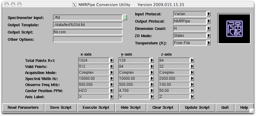
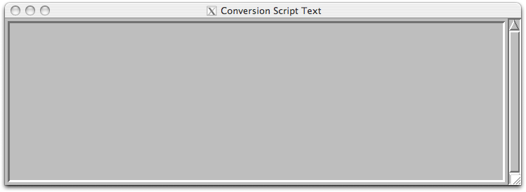
Step 1: Under the same directory where the procpar and fid files are, type ‘varian’ and this will start a tcl/tk script that brings up two windows.
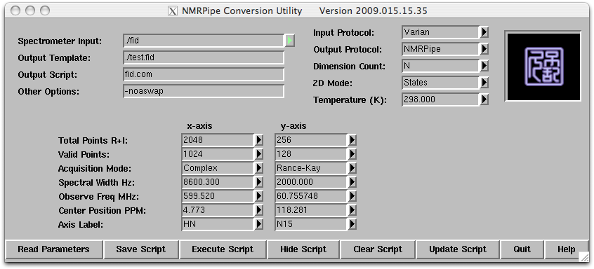
Step 2: Click on the ‘Read Parameters’ button and the script will read the parameter file (‘procpar’) and update the parameters.
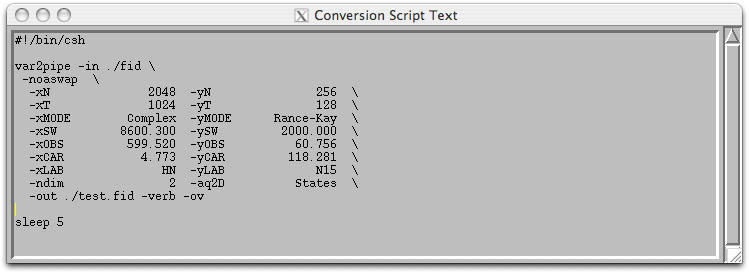
The template shows parameters for two dimensions x and y. The x dimension is the direct dimension and is always collected as complex data (quadrature detection) and the xMODE is set as complex. The xN (real+imaginary points) parameter is twice the xT (complex points) parameter. For the indirect dimension y, the yN parameter is twice the yT parameter (number of increments, ni for a Varian instrument), indicating that we are collecting complex dataset to account for ‘quadrature’ in the indirect dimension. For the sensitivity-enhanced experiments the yMODE will be set to “Rance-Kay”. The frequency values can be modified using the pull down tab. The center position ppm of each dimension (xCAR and yCAR) can be updated at this stage and it can also be update later.
Step 3: Click on ‘Save Script’, and the ‘Execute Script’. A converted dataset in NMRPipe format will be created as test.fid along with an UNIX shell script called ‘fid.com’. All of the processing parameters and the location of the input and output files are store in the ‘fid.com’ script and it can be modified using a text editor.
Processing and Visualizing 2D Dataset
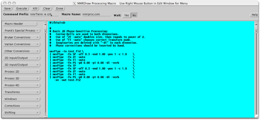
Similar to the conversion script, all of the commands for data processing are also complied into a script file (brief summaries of the commands). The nmrDraw program has a macro-editing tool to aid in the construction of script. The nmrDraw program can be launch by typing ‘nmrDraw &’ under the same directory the dataset is. The macro editor can be started by selecting ‘Macro Edit’ from the ‘File’ menu. This editor contains build in macros to process 2D, 3D, and 4D dataset, or it can create lines of text for various functions. The script can be saved and executed inside the macro editor.
An alternative way to create a processing script is to copy an existing one and edit it with a text editor. An example of processing script for a 2D 15N HSQC spectrum is shown below. The script starts off by reading in the time domain data ‘test.fid’ using the ‘nmrPipe –in’ command following by ‘\’ at the end of each line. Each subsequent ‘nmrPipe –fn’ command line will begin with a unix ‘|’ and end with ‘\’. A solvent suppression filter SOL was first applied to removed residual solvent followed by a 90 degrees sine bell squared apodization (equivalent to cosine) with scale factor for first point as 0.5. The data is then zero-filled to the nearest power of 2, Fourier transformed, phased, and the amide region of the spectrum (left half) extracted. The TP functions transpose the data to the y-axis to apply linear prediction, apodization, zero fill, Fourier transform, phasing to the y-dimension, and output the finished file as ‘test.ft2’. When the first point is collected at a half dwell time (for a Varian instrument, f1180=’y’), the phasing values in the indirect dimension are set to ‘-90 for p0 and 180 for p1’ and the first point multiplier set to 1.0.
|nmrPipe  -in test.fid                                            \
| nmrPipe -fn SOL                                               \ ## Solvent suppresion
| nmrPipe  -fn SP -off 0.5 -end 1.00 -pow 2 -c 0.5  \ ## Apodization
| nmrPipe  -fn ZF -auto                                        \ ## Zero fill
| nmrPipe  -fn FT -auto                                        \ ## Fourier transformation
| nmrPipe -fn PS -p0 13.6 -p1 0.0  -di                    \ ## Phase correction
| nmrPipe  -fn EXT –left –sw                                \ # Extract spectrum
| nmrPipe -fn TP                                                 \ ## Transpose to the y-axis
| nmrPipe -fn LP -fb                                             \ ## Add liner prediction
| nmrPipe -fn SP -off 0.5 -end 0.98 -pow 2 -c 1.0    \
| nmrPipe -fn ZF -auto                                          \
| nmrPipe -fn FT -auto                                          \
| nmrPipe -fn PS -p0 -90.0 -p1 180.0   -di               \
| nmrPipe -fn TP                                                  \
| nmrPipe –out test.ft2  -verb 2 -ov
Suggested Workflow
Step 1: Generate the processing script with the appropriate commands and functions using the macro editor or modifying an existing script. Set both the p0 and p1 phasing values of the direct dimension to 0.
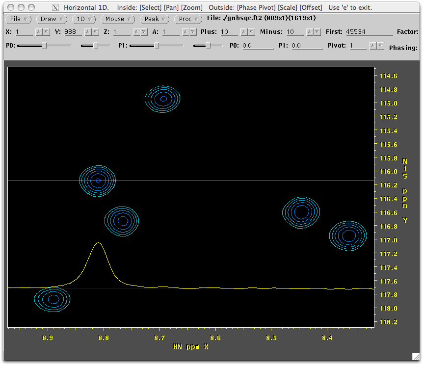
Step 2: Execute the processing script in a UNIX terminal. Load the spectrum into nmrDraw to perform phase correction and optimize the applied functions. A 1D horizontal trace can be activate by typing ‘h’ in the spectrum window and the phase of the dimension can be adjusting using the P0 and P1 slider bars. To phase an indirect dimension, type 'v'. Now the P0 and P1 slider bars will change the phase of the indirectly-detected dimension.
Step 3: Execute the processing script with optimized parameters.
Step 4: Convert the processed data to the format of graphical NMR assignment program.
Updated by Hsiau-Wei Lee, 2011
