Resonance Assignment/Sparky: Difference between revisions
No edit summary |
m (moved Sparky to Resonance Assignment/Sparky) |
||
| (5 intermediate revisions by one other user not shown) | |||
| Line 5: | Line 5: | ||
Sparky is a software package developed at the University of San Francisco for visualizing and analyzing multidimensional (2D, 3D or 4D) NMR spectra. Sparky plays a critical role as the link between spectral data and assignment/structure determination programs. The input for the program is processed spectra from various formats (NMRPipe, Felix, Varian or Bruker) converted into Sparky (i.e., “ucsf” format) via processing scripts supplied with the program. One can output a variety of data from Sparky including: chemical shift assignments, peak lists, and post script images of spectra. In the following sections we describe the practical aspects of using Sparky and standard approaches employed by NESG researchers using this program in structure determination projects. A descriptive on-line manual for a recent Sparky version (3.115) is available at: [http://www.cgl.ucsf.edu/home/sparky/manual/index.html www.cgl.ucsf.edu/home/sparky/manual/index.html]. | Sparky is a software package developed at the University of San Francisco for visualizing and analyzing multidimensional (2D, 3D or 4D) NMR spectra. Sparky plays a critical role as the link between spectral data and assignment/structure determination programs. The input for the program is processed spectra from various formats (NMRPipe, Felix, Varian or Bruker) converted into Sparky (i.e., “ucsf” format) via processing scripts supplied with the program. One can output a variety of data from Sparky including: chemical shift assignments, peak lists, and post script images of spectra. In the following sections we describe the practical aspects of using Sparky and standard approaches employed by NESG researchers using this program in structure determination projects. A descriptive on-line manual for a recent Sparky version (3.115) is available at: [http://www.cgl.ucsf.edu/home/sparky/manual/index.html www.cgl.ucsf.edu/home/sparky/manual/index.html]. | ||
| | ||
== ''' | == '''Methods''' == | ||
==== Conversion of processed spectra to Sparky input format ==== | ==== Conversion of processed spectra to Sparky input format ==== | ||
| Line 20: | Line 20: | ||
ucsfdata –p1 –o output.ucsf input.ucsf | ucsfdata –p1 –o output.ucsf input.ucsf | ||
</pre> | </pre> | ||
==== Launching Sparky ==== | ==== Launching Sparky ==== | ||
| Line 34: | Line 33: | ||
===== Figure 1: Spectral views in Sparky ===== | ===== Figure 1: Spectral views in Sparky ===== | ||
[[Image:Sparky fig1.png|1200x800px]] | [[Image:Sparky fig1.png|1200x800px]] | ||
==== Peak Picking<br> ==== | ==== Peak Picking<br> ==== | ||
| Line 42: | Line 41: | ||
===== Figure 2: Restricted peak pick box ===== | ===== Figure 2: Restricted peak pick box ===== | ||
[[Image:Sparky kr.png]] | [[Image:Sparky kr.png]] | ||
==== Manipulating and Analyzing Multiple Spectra<br> ==== | ==== Manipulating and Analyzing Multiple Spectra<br> ==== | ||
| Line 50: | Line 49: | ||
===== Figure 3: Backbone spectra for a single spin system ===== | ===== Figure 3: Backbone spectra for a single spin system ===== | ||
[[Image:Sparky BB.png|1200x700px]] | [[Image:Sparky BB.png|1200x700px]] | ||
==== Assignment and Peak Lists<br> ==== | ==== Assignment and Peak Lists<br> ==== | ||
| Line 74: | Line 73: | ||
The peaks2sparky.awk script can be obtained at: | The peaks2sparky.awk script can be obtained at: | ||
[http://www.nmr.chem.uu.nl/~eiso/help/index.html www.nmr.chem.uu.nl/~eiso/help/index.html] <br> | [http://www.nmr.chem.uu.nl/~eiso/help/index.html www.nmr.chem.uu.nl/~eiso/help/index.html] <br> | ||
==== Common Sparky Commands<br> ==== | ==== Common Sparky Commands<br> ==== | ||
| Line 82: | Line 81: | ||
a1, a2, a3: add SW to peak in F1, F2, F3 dimension; for aliased spectra<br>A1, A2, A3: subtract SW from peak in F1, F2, F3 dimension; for aliased spectra<br>at: assignment tool; for assigning a peak<br>cl: adjust colour of ornament<br>ct: adjust contour levels and colours:<br>dr: delete resonances not used in any peak assignment (cleans up resonance list)<br>eu: undo last peak manipulation<br>it: integration tool<br>kr: restrictive peak picking tool<br>lt: opens the peak list for a given spectrum; various options in here<br>oc: ornament copy; for copying assignment/label information between spectra<br>ol: overlay views; useful for comparing spectra<br>op: ornament paste<br>oz: adjust size of ornament<br>pa: select all peaks in a spectrum<br>pc: peak center<br>pv: list of sizes and peak counts in all open spectra<br>rl: resonance list for the project; various functions and displays in there<br>rp: read in a list of peaks in sparky format (i.e. from AutoAssign or PINE)<br>rr: resonance rename<br>st: spectrum tool; useful for global axes shift corrections<br>tb: table of resonances for the project: useful for seeing missing assignments<br>vc: view centering; useful for going to a specific peak in a 3D selected in a 2D<br>vd: view duplicate; duplicate view of a spectrum into another window<br>vR: show assignments on edge of spectrum<br>vS: show 1D slice on edge of spectrum<br>vt: view settings; a variety of spectral settings including aspect ratio<br>xa: show nucleus type on axis<br>xe: special Python command for saving peak list in xeasy format<br>xr: roll axes; useful for 3D and 4D spectra<br>xx: axis transpose<br>yt: synchronize axes of various spectra: useful for analyzing series of 3D’s<br>zf, zi, zo, zp: zoom full spectrum, zoom in, zoom out, zoom previous<br><br>Commonly used pointer modes (for the mouse):<br> F1: selection mode<br> F6: add a label<br> F7: add a line<br> F8: peak picking mode<br> F10: integration mode<br> F11: zoom mode | a1, a2, a3: add SW to peak in F1, F2, F3 dimension; for aliased spectra<br>A1, A2, A3: subtract SW from peak in F1, F2, F3 dimension; for aliased spectra<br>at: assignment tool; for assigning a peak<br>cl: adjust colour of ornament<br>ct: adjust contour levels and colours:<br>dr: delete resonances not used in any peak assignment (cleans up resonance list)<br>eu: undo last peak manipulation<br>it: integration tool<br>kr: restrictive peak picking tool<br>lt: opens the peak list for a given spectrum; various options in here<br>oc: ornament copy; for copying assignment/label information between spectra<br>ol: overlay views; useful for comparing spectra<br>op: ornament paste<br>oz: adjust size of ornament<br>pa: select all peaks in a spectrum<br>pc: peak center<br>pv: list of sizes and peak counts in all open spectra<br>rl: resonance list for the project; various functions and displays in there<br>rp: read in a list of peaks in sparky format (i.e. from AutoAssign or PINE)<br>rr: resonance rename<br>st: spectrum tool; useful for global axes shift corrections<br>tb: table of resonances for the project: useful for seeing missing assignments<br>vc: view centering; useful for going to a specific peak in a 3D selected in a 2D<br>vd: view duplicate; duplicate view of a spectrum into another window<br>vR: show assignments on edge of spectrum<br>vS: show 1D slice on edge of spectrum<br>vt: view settings; a variety of spectral settings including aspect ratio<br>xa: show nucleus type on axis<br>xe: special Python command for saving peak list in xeasy format<br>xr: roll axes; useful for 3D and 4D spectra<br>xx: axis transpose<br>yt: synchronize axes of various spectra: useful for analyzing series of 3D’s<br>zf, zi, zo, zp: zoom full spectrum, zoom in, zoom out, zoom previous<br><br>Commonly used pointer modes (for the mouse):<br> F1: selection mode<br> F6: add a label<br> F7: add a line<br> F8: peak picking mode<br> F10: integration mode<br> F11: zoom mode | ||
<br> | <br> | ||
==== Example Protein Assignment Project<br> ==== | ==== Example Protein Assignment Project<br> ==== | ||
| Line 97: | Line 96: | ||
[[Image:Sparky Fig6b.png|800x500px]] | [[Image:Sparky Fig6b.png|800x500px]] | ||
c. Preparation of final bmrb file<br>For the most precise chemical shifts it is recommended that a final resonance list file (made by “rl”) be generated based on a subset of assigned spectra (2D NH-HSQC, 2D CH-HSQC aliphatic and aromatic, 3D HNCO and 3D HN(CA)CO; alternatively, the carbonyl spectra can be omitted and those assignments can be added to the bmrb file later). If one begins from a larger project and deletes other spectra, use the “dr” command to delete any unused assignments. Also, try to avoid using “Q” in your assignment nomenclature in this subset of spectra. Check the standard deviations in the resonance list for any unusually high values, to be sure there are no incorrect assignments. This resonance list is then converted to a bmrb using the “sparkyRL2bmrb.pl” script as described above. Prior to moving on to structure determination programs, it is advisable to check the bmrb file for any missing or unusual shifts/typos using the AVS scripts, “missing_shifts.pl” and “validate_assignments.pl”. <br> | c. Preparation of final bmrb file<br>For the most precise chemical shifts it is recommended that a final resonance list file (made by “rl”) be generated based on a subset of assigned spectra (2D NH-HSQC, 2D CH-HSQC aliphatic and aromatic, 3D HNCO and 3D HN(CA)CO; alternatively, the carbonyl spectra can be omitted and those assignments can be added to the bmrb file later). If one begins from a larger project and deletes other spectra, use the “dr” command to delete any unused assignments. Also, try to avoid using “Q” in your assignment nomenclature in this subset of spectra. Check the standard deviations in the resonance list for any unusually high values, to be sure there are no incorrect assignments. This resonance list is then converted to a bmrb using the “sparkyRL2bmrb.pl” script as described above. Prior to moving on to structure determination programs, it is advisable to check the bmrb file for any missing or unusual shifts/typos using the AVS scripts, “missing_shifts.pl” and “validate_assignments.pl”. <br> | ||
== ''' | == '''References''' == | ||
When using Sparky in your structure determination please cite:<br> T.D. Goddard & D.G. Kneller, SPARKY 3,<br> University of California, San Francisco<br> | When using Sparky in your structure determination please cite:<br> T.D. Goddard & D.G. Kneller, SPARKY 3,<br> University of California, San Francisco<br> | ||
| Line 105: | Line 104: | ||
<br> | <br> | ||
<br> <br> <br> | |||
<br> | <br> | ||
Latest revision as of 23:22, 5 January 2010
Sparky
Introduction
Sparky is a software package developed at the University of San Francisco for visualizing and analyzing multidimensional (2D, 3D or 4D) NMR spectra. Sparky plays a critical role as the link between spectral data and assignment/structure determination programs. The input for the program is processed spectra from various formats (NMRPipe, Felix, Varian or Bruker) converted into Sparky (i.e., “ucsf” format) via processing scripts supplied with the program. One can output a variety of data from Sparky including: chemical shift assignments, peak lists, and post script images of spectra. In the following sections we describe the practical aspects of using Sparky and standard approaches employed by NESG researchers using this program in structure determination projects. A descriptive on-line manual for a recent Sparky version (3.115) is available at: www.cgl.ucsf.edu/home/sparky/manual/index.html.
Methods
Conversion of processed spectra to Sparky input format
Typically we process NMR spectra using NMRPipe, hence it is necessary to convert the spectra from pipe to ucsf format using the following command:
pipe2ucsf [options] filename.pipe filename.ucsf
For higher dimensional spectra a flag can be used to swap the dimension order if desired. For example “-213” swaps the order of the 1st and 2nd indirect dimensions of a 3D spectrum. This is applicable to many Varian 3D triple resonance spectra.
Another useful function is making 2D projections of higher dimensional spectra. This is done using the “ucsfdata” command. First, run the following command:
ucsfdata filename.ucsf
to obtain a list of information for each dimension of the spectrum. Then, for example, to make a 2D F23 projection of a 3D spectrum use:
            ucsfdata –s1 [# points] –r –o output.ucsf input.ucsf
        or
            ucsfdata –p1 –o output.ucsf input.ucsf
Launching Sparky
To open a spectrum for the first time use:
sparky filename.ucsf
To open a single save file or project (a collection of save files) use:
            sparky filename.save

            sparky filename.proj
If using Sparky for the first time, a Sparky folder will be automatically generated in your home directory, with various subfolders. It is recommended that spectral (.ucsf), save and project files for a specific project be stored and launched from a specific directory in order to avoid confusion between multiple protein projects. The .save and .proj files are simple text files which contain links pointing to where data (.ucsf and .save files) are located on your machine. If a spectrum fails to open check the links in these files.
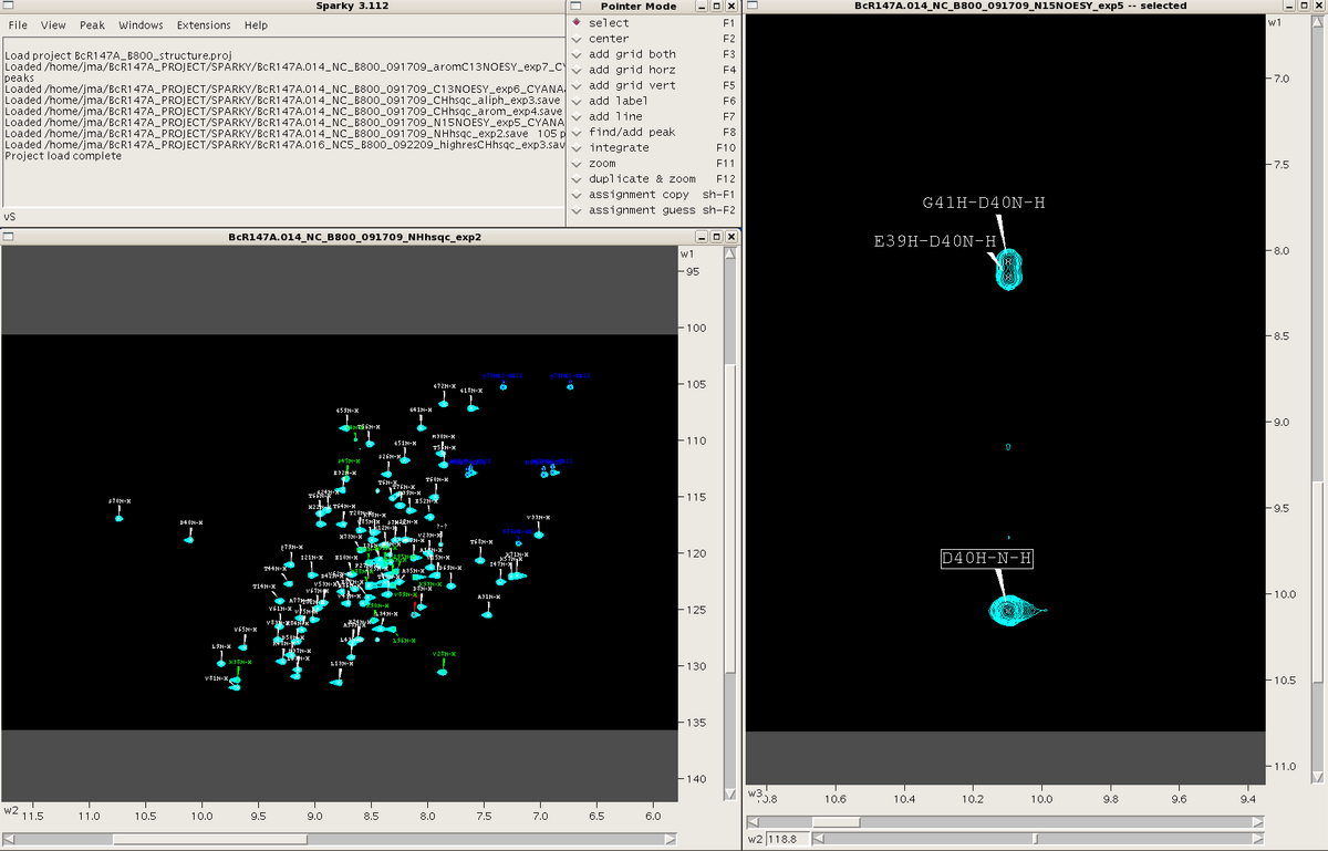
When Sparky is launched a menu box appears. This box tracks all commands performed during a session. One can make commands in Sparky using the mouse and clicking various commands under the different menus within the menu box or by using a plethora of two-letter “accelerators”. A “pointer mode” box also opens at the start of a session and allows the user to toggle between various pointer modes. Spectra are launched in individual windows. See Figure 1. All spectra are opened as 2D planes, with the additional dimension(s) of 3D and 4D spectra represented by sliders along the bottom of the spectral window.
Figure 1: Spectral views in Sparky
Peak Picking
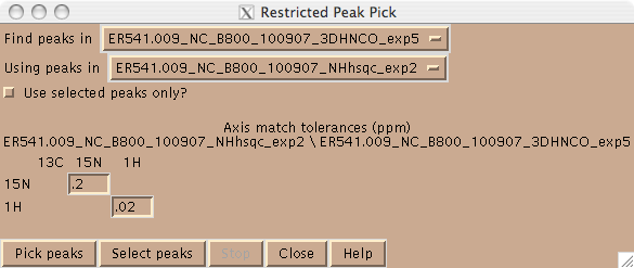
Peaks can be picked in Sparky in one of two ways. One can use the left mouse button in peak picking mode (F8). In this mode one drags the mouse over the peak(s) in the spectrum and Sparky will place a peak at the maximum intensity. One can also place a peak using the left mouse button; this is desirable in cases where there is substantial peak overlap. Alternatively, one can pick peaks in a higher dimensional spectrum using peaks in a lower dimensional spectrum using the restricted peak picking command “kr” and user defined tolerances (Figure 2). In this mode, be sure to set the contour levels in the target spectrum to an appropriate level using the “ct” command, in order to avoid picking a lot of noise.
Figure 2: Restricted peak pick box
Manipulating and Analyzing Multiple Spectra
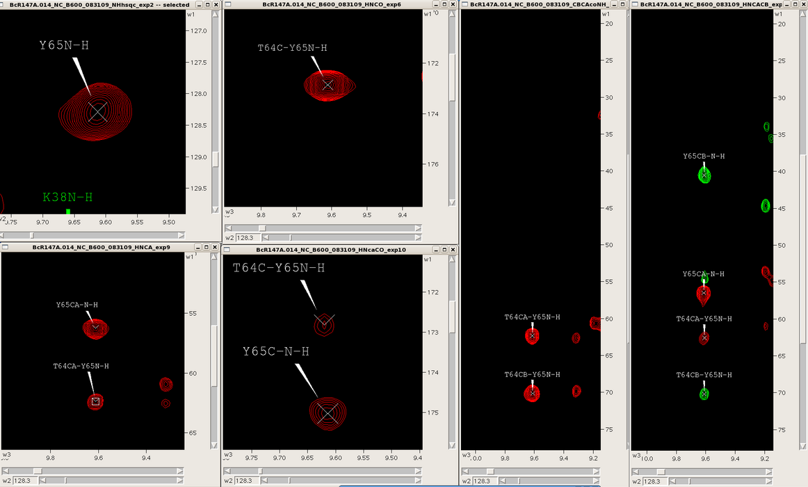
One can easily navigate through multiple spectra in Sparky, particularly spectra with common root dimensions (i.e., NH). For example, in the case of backbone resonance assignment with conventional triple resonance approaches one can synchronize 3D spectra (i.e., HNCO, HNcoCA, HNCA, HNcaCO, CBCAcoNH, HNCACB, HBHAcoNH) to each other and the NH-HSQC using the “yt” command, and then jump to successive NH-roots using the “vc” command (Figure 3). Similarly, one can use this approach to synchronize and navigate between entire spin systems in 3D side chain experiments (i.e., CCH-TOCSY, HCCH-TOCSY, HCCH-COSY) as well as NOESY spectra (i.e., 3D 15N-filtered and 13C-filtered NOESYs, and 4D 13C-13C-NOESY).
Figure 3: Backbone spectra for a single spin system
Assignment and Peak Lists
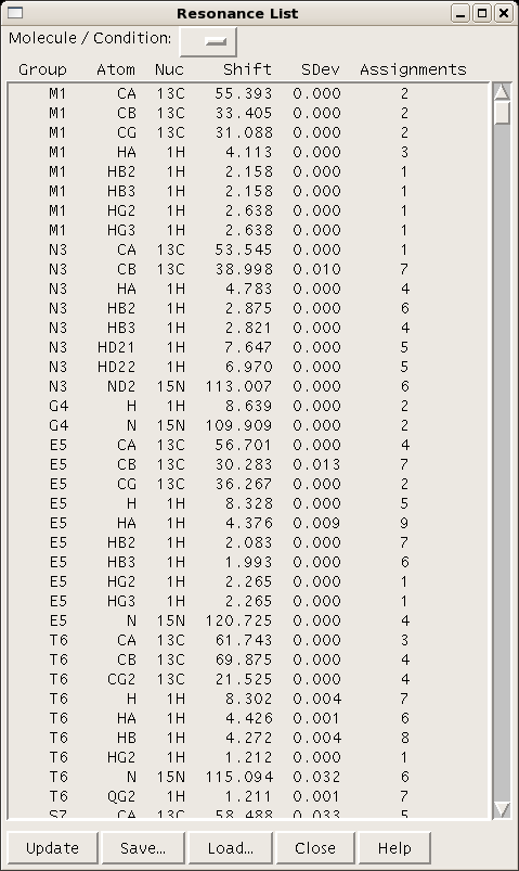
A table of resonance lists for a given project can be generated using the command “rl” (Figure 4).
Figure 4: Sparky resonance list
This list can be saved and subsequently converted to bmrb format using a script in the AutoAssign/bin directory.
            sparkyRL2bmrb.pl input_rl output_bmrb sequence_start sequence [options]

            options:  -diastereo –unique_methyls –bmrb2
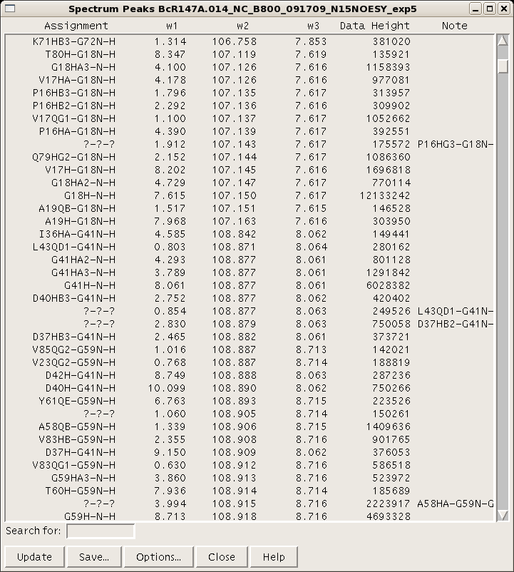
Each resonance value is an average of all the assignments for that resonance across all open spectra. Therefore, be sure that the assignment nomenclature used throughout the project is consistent. A peak list for a given spectrum can be generated and using the command “lt”. (Figure 5). There are various options for column visualization and ordering, and the list can be saved for input into AutoAssign or AutoStructure. For input into CYANA, NOESY spectral peak lists can be generated in XEASY format using the “xe” command.
Figure 5: Sparky peak list
Assigned backbone peak lists from AutoAssign or PINE, and assigned NOESY peak lists from AutoStructure can be easily read back into the appropriate spectra using the “rp” command. In the case of CYANA peak lists one must convert the peak list back into Sparky using the following command:
awk –f peaks2sparky.awk file.seq file.prot file_cycle7.peaks > assigned_4sparky.list
The peaks2sparky.awk script can be obtained at:
www.nmr.chem.uu.nl/~eiso/help/index.html
Common Sparky Commands
There are numerous useful two-letter commands that can speed up spectral analysis in Sparky. Here is a list of commonly used accelerators:
a1, a2, a3: add SW to peak in F1, F2, F3 dimension; for aliased spectra
A1, A2, A3: subtract SW from peak in F1, F2, F3 dimension; for aliased spectra
at: assignment tool; for assigning a peak
cl: adjust colour of ornament
ct: adjust contour levels and colours:
dr: delete resonances not used in any peak assignment (cleans up resonance list)
eu: undo last peak manipulation
it: integration tool
kr: restrictive peak picking tool
lt: opens the peak list for a given spectrum; various options in here
oc: ornament copy; for copying assignment/label information between spectra
ol: overlay views; useful for comparing spectra
op: ornament paste
oz: adjust size of ornament
pa: select all peaks in a spectrum
pc: peak center
pv: list of sizes and peak counts in all open spectra
rl: resonance list for the project; various functions and displays in there
rp: read in a list of peaks in sparky format (i.e. from AutoAssign or PINE)
rr: resonance rename
st: spectrum tool; useful for global axes shift corrections
tb: table of resonances for the project: useful for seeing missing assignments
vc: view centering; useful for going to a specific peak in a 3D selected in a 2D
vd: view duplicate; duplicate view of a spectrum into another window
vR: show assignments on edge of spectrum
vS: show 1D slice on edge of spectrum
vt: view settings; a variety of spectral settings including aspect ratio
xa: show nucleus type on axis
xe: special Python command for saving peak list in xeasy format
xr: roll axes; useful for 3D and 4D spectra
xx: axis transpose
yt: synchronize axes of various spectra: useful for analyzing series of 3D’s
zf, zi, zo, zp: zoom full spectrum, zoom in, zoom out, zoom previous
Commonly used pointer modes (for the mouse):
F1: selection mode
F6: add a label
F7: add a line
F8: peak picking mode
F10: integration mode
F11: zoom mode
Example Protein Assignment Project
a. Backbone assignments
When starting an assignment project on a specific protein it is recommended that all Sparky files are collected in a specific project directory. In a conventional triple resonance backbone assignment one matches intraresidue and sequential C’, Cα, and Cβ resonances in 2D NH-HSQC and 3D HNCO, HN(CA)CO, CBCA(CO)NH, and HNCACB, for example (Figure 3, above). For automated backbone assignment using programs such as AutoAssign or the PINE server (http://miranda.nmrfam.wisc.edu/PINE/) it is important that the peak lists are properly registered to each other, particularly in the N and HN dimensions. Any systematic shifting between spectra can be corrected using the “st” command. Peak lists should contain chemical shift information in each dimension and the peak intensities. For input into AutoAssign, additional spin system information can be specified in the Notes column; in the case of PINE, one should remove this column. Assigned peak lists in Sparky format from either AutoAssign or PINE can be read back into the spectra using the “rp” command. One can then check the assignments for each NH spin system using the “vc” command, using the NH-HSQC as the root spectrum. One can also fill in the Hα and Hβ assignments in the HBHA(CO)NH spectrum. At this stage one can make a preliminary bmrb file (using the “rl” and “sparkyRL2bmrb.pl” script), and use this to make a CH-HSQC list containing predicted resonance assignments using the “bmrbACS2SparkyPks.pl” script as follows:
bmrbACS2SparkyPks.pl file.bmrb output.list CA HA
This outputs a list of CA-HA assignments in Sparky peak list format. One can write a script with lines in the above format for other CH-HSQC resonance types (I.e., CA-HA2, CA-HA3, etc.) and concatenate the output files into one list for import back into Sparky.
b. Side chain assignments
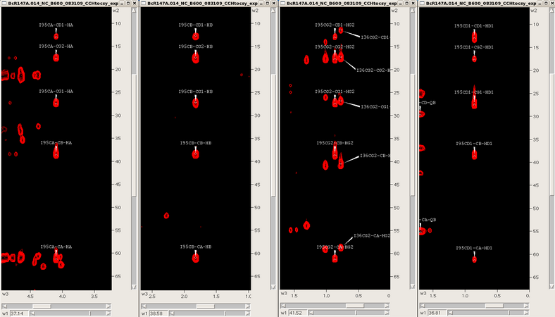
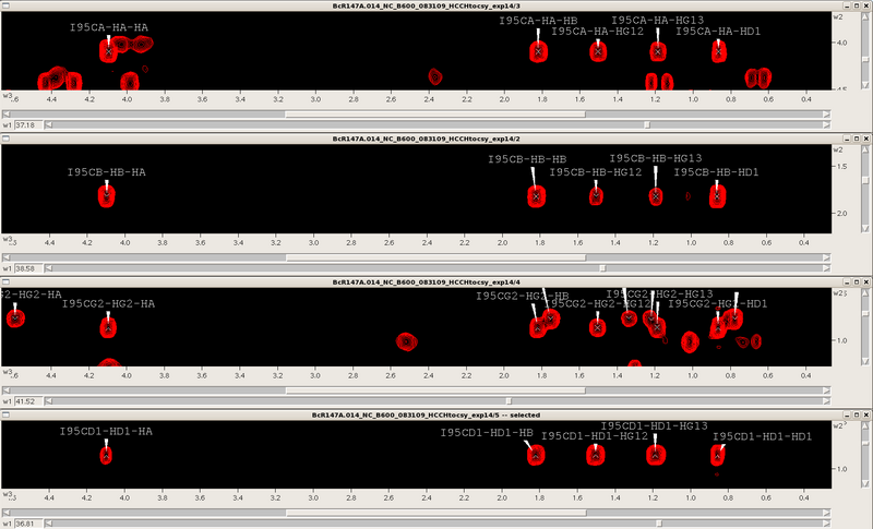
Starting from the assigned alpha and beta cross-peaks in the CH-HSQC one then extends the assignment process into the aliphatic side chains using the 3D HCCH-TOCSY, CCH-TOCSY and HCCH-COSY spectra synchronized with the CH-HSQC. For example, for an isoleucine spin system one skips from one carbon to the next finding the same TOCSY pattern for that spin system (see Figure 6). Assignments are manually placed back into the CH-HSQC spectrum until the aliphatic assignment is complete. Additional side chain information through the NH roots can be obtained from the 3D CC(CO)NH TOCSY if necessary. Aromatic and side chain NH2 assignments are typically obtained by NOESY spectra, and stereospecific methyl assignments (Leu/Val) are obtained from a high resolution CH-HSQC spectrum of a fractionally 13C-labeled protein sample.
Figure 6: TOCSY slices for an isoleucine (α,β,γ2,δ1)
c. Preparation of final bmrb file
For the most precise chemical shifts it is recommended that a final resonance list file (made by “rl”) be generated based on a subset of assigned spectra (2D NH-HSQC, 2D CH-HSQC aliphatic and aromatic, 3D HNCO and 3D HN(CA)CO; alternatively, the carbonyl spectra can be omitted and those assignments can be added to the bmrb file later). If one begins from a larger project and deletes other spectra, use the “dr” command to delete any unused assignments. Also, try to avoid using “Q” in your assignment nomenclature in this subset of spectra. Check the standard deviations in the resonance list for any unusually high values, to be sure there are no incorrect assignments. This resonance list is then converted to a bmrb using the “sparkyRL2bmrb.pl” script as described above. Prior to moving on to structure determination programs, it is advisable to check the bmrb file for any missing or unusual shifts/typos using the AVS scripts, “missing_shifts.pl” and “validate_assignments.pl”.
References
When using Sparky in your structure determination please cite:
T.D. Goddard & D.G. Kneller, SPARKY 3,
University of California, San Francisco
