Processing non-uniformly sampled spectra with Multidimensional Decomposition: Difference between revisions
No edit summary |
No edit summary |
||
| Line 23: | Line 23: | ||
<br>[[Image:MDDGUIstep2.jpg|thumb|left|505px]][[Image:MDDGUIstep2 out.jpg|thumb|right|505px]]<br> | <br>[[Image:MDDGUIstep2.jpg|thumb|left|505px]][[Image:MDDGUIstep2 out.jpg|thumb|right|505px]]<br> | ||
==== Step 3. Process the first plane <br> ==== | ==== Step 3. Process the first plane <br> ==== | ||
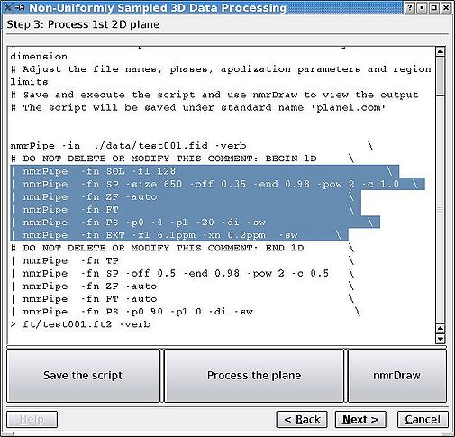
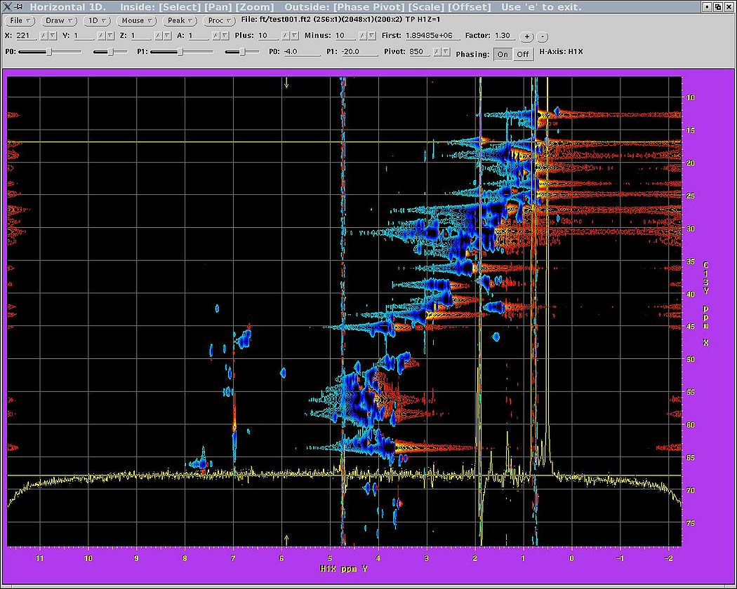
For the Bruker data, the first plane is regularly sampled while for Varian it is not, which may make this step more difficult for Varian data. One only needs to adjust phasing, apodisation, region of interest and other parameters for the '''acquisition '''dimension. The better the phasing, the better the convergence and the fewer the artefacts. It will be difficult to change the acquisition dimension parameters afterwards without redoing the calculation, so spend a few rounds with NMRDraw until you are happy and the phases are set properly. As usual, click "Save", then "Run" each time you want to reprocess the plane. Button "nmrDraw" simply calls that program. | For the Bruker data, the first plane is regularly sampled while for Varian it is not, which may make this step more difficult for Varian data. One only needs to adjust phasing, apodisation, region of interest and other parameters for the '''acquisition '''dimension. The better the phasing, the better the convergence and the fewer the artefacts. It will be difficult to change the acquisition dimension parameters afterwards without redoing the calculation, so spend a few rounds with NMRDraw until you are happy and the phases are set properly. As usual, click "Save", then "Run" each time you want to reprocess the plane. Button "nmrDraw" simply calls that program. | ||
<br> | |||
[[Image:MDDGUIstep3.jpg|thumb|left|505px]][[Image:MDDGUIstep3_final.jpg|thumb|right|505px]] | |||
[[Image:MDDGUIstep3_plane.jpg|thumb|1050px]] | |||
<br> | <br> | ||
Revision as of 19:02, 24 November 2009
Introduction and Prerequisites
This section gives a step-by-step manual to processing with the MDDGUI program, developed in the Arrowsmith lab (University Health Network and University of Toronto). It is designed for processing 3D spectra collected with non-uniform or non-linear sampling (NUS). The spectra can be collected either on Varian spectrometers with later versions of BioPack installed (click here for the relevant guide for Varian spectrometers) or on Bruker spectrometers running TopSpin (click here for the Arrowsmith protocol for NUS data collection on Bruker instruments).
The GUI package uses the mddnmr software developed by Vladislav Orekhov (Swedish NMR Centre, University of Gothenburg, http://www.nmr.gu.se/~mdd). Please contact him for your copy of the software. The GUI can be downloaded here or requested from the Arrowsmith group. You need Qt libraries in order to compile the GUI, or you can use the precompiled Linux version. Please refer to the installation README file for details. In addition to these two packages, you should have working nmrPipe and nmrDraw programs, as apodization, Fourier transforms, etc are performed by nmrPipe.
Processing with MDDGUI
Before the Multi-dimensional decomposition can be started, the raw data has to be converted through a number of steps to an appropriate format. The steps below are accompanied by the GUI screen shots. To move between the different stages of the processing, use "Next" and "Back" buttons. Refer to README file or tutorial for more specific instructions.
Step 1. Reshuffle FIDs
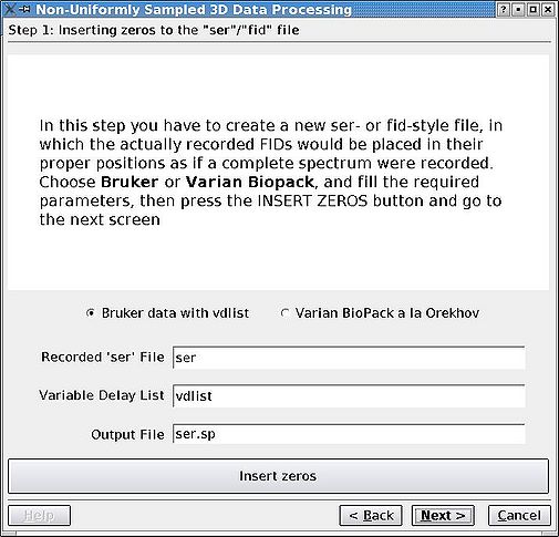
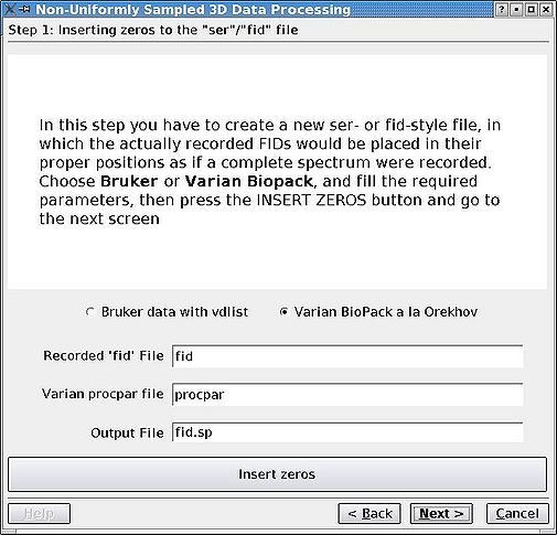
Rearrange the FIDs in the ser of fid file so that they are in correct positions for an imaginary case as if the data set was sampled regularly. The missing FIDs are replaced by zeros as dictated by the vdlist or procpar files. First, click the appropriate radio button, edit any file names if necessary, and click Insert Zeros before proceeding.
Step 2. Convert to NMRPipe format
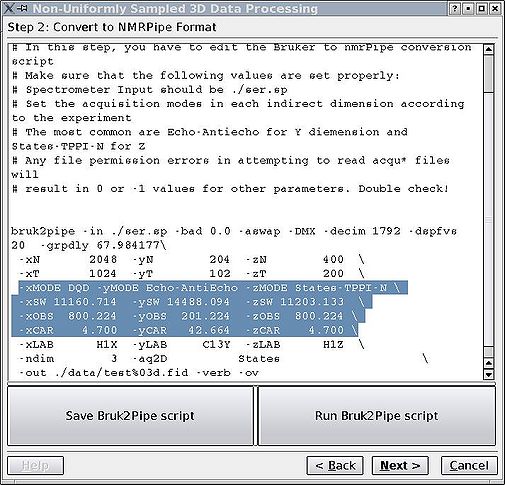
In this step there are a few parameters that the GUI might read wrong, especially with later versions of TopSpin. You can edit it as a simple bruk2pipe script. Pay extra attention to carrier and spectrometer frequencies, matrix sizes and acquisition modes (highlighted). In TopSpin2.1 we discovered that sweep width is sometimes not recorded in the acqu* files, therefore check that as well. Click Save, then Run.
NB! Make sure the spectrometer input is the reshuffled file (.sp)!
Step 3. Process the first plane
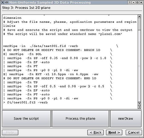
For the Bruker data, the first plane is regularly sampled while for Varian it is not, which may make this step more difficult for Varian data. One only needs to adjust phasing, apodisation, region of interest and other parameters for the acquisition dimension. The better the phasing, the better the convergence and the fewer the artefacts. It will be difficult to change the acquisition dimension parameters afterwards without redoing the calculation, so spend a few rounds with NMRDraw until you are happy and the phases are set properly. As usual, click "Save", then "Run" each time you want to reprocess the plane. Button "nmrDraw" simply calls that program.
Step 4. Processing the acquisition dimension
Using the parameters from step 3, Fourier transform (FT) the acquisition dimension only for the whole data set and extract the region of interest.
Step 5. Converting to MDD format
Divide the the partially Fourier transformeded but still sparse spectrum into a number of regions overlapping by their acquisition dimension and convert these regions to MDD format. This is the step before proceeding to calculations themselves. Make sure you select "Multiregion" radiobutton. Parallel computation is becoming obsolete, although is supported for now.
Step 6. Run MDD
As simple as that. Check README for more detailed instructions. You might need to do some editing of the "runmdd.sh" script depending on cluster availability (e.g., you may need to remove & from the mddnmr command if your calculation is running on a desktop). In the Arrowsmith group, we usually open a separate terminal window, login to our cluster and start the claculation from there. Don't close the GUI in the meantime. If you do, it is a bit tricky to restart from where you are.
Step 7. Reconstructing the spectrum
Using the output of MDD, replace the zeros ( i.e. missing FIDs) by the reconstructed values. Here, if you had the GUI open through the previous step, the values will be filled automatically. If you did close it, go to step 5, choose "Multiregion" radiobutton, proceed to step 7 and fill out the values. That was the tricky part.
Step 8. Fourier transform of indirect dimensions
Here the task is purely NMRPipe. Do to your indirect dimensions what you need to do. You may need to play around with "FT -auto" if your peaks are not making sense. That is mainly because the GUI can't easily distiguish between "Complex", "States-TPPI" and related modes. So you may need to change the FT flags to rectify. Plus, you don't need the GUI anymore, that is the final step and you can edit the script to your liking.
README.pdf: PDF of the README for the processing package
