.
It is not reauired this peak list to be referenced.
:: Set tolerances for chemical shift matching in different spectral dimensions.
The name of the saved file and it’s location are specified by user.
♦ Specified tolerances.
There are two steps in executing this command.
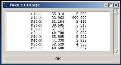
User can use the information shown in the main FMCGUI window and check /edit the list in the entry section of “fake C13HSQC” window accordingly.
Pressing OK will result in loading the peak list from the entry window into memory as C13HSQC peak list.
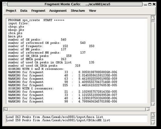
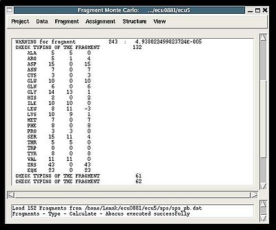
The warning messages of the command are shown in the main FMCGUI window (see for example, Figure 2.4).
.
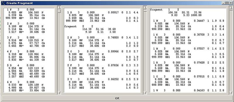
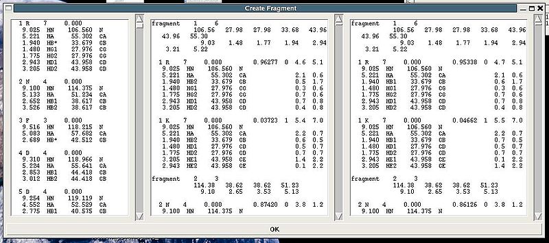
"Create Fragment" window consists of three sections. The left sections contains suggested bPB fragments, while the other sections contains two reports of fragments scoring with both C and H resonances and with only C resonances, respectively. Following the warning messages shown in the main FMCGUI window (see Figure 2.4), user can accept/modify generated bPB fragments. Alternatively, when ‘poor’ bPB fragments are present, user can go back to spectra, fix the pick lists accordingly, and repeat the fragment generation again.
:: Create and avaluate PB fragments.
( As an option, HNCA peak list could be not referenced as well)
♦ Specified tolerances.
A number of PB fragments corresponding to 20 different amino acid types are generated from user-identified spin-systems. Each generated PB fragment is evaluated by a score S (see Figure 1.2) that measure how good the spin-system chemical shifts match corresponding statistical chemical shifts derived from BMRB database. The PB fragment with highest score is selected to form a list of PB fragments.
.
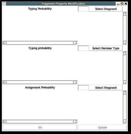
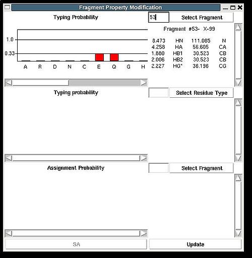
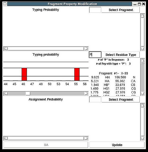
The command opens "Fragment Property Modification" (FPM) window (see Figure).
♦ loaded HNCO, CBCACONH, and HNCA peak lists.
♦ specified tolerances.
♦ chemical shift names are corrected for assigned PB-fragments (the fragments with A_id > -99 )
Assignment>Contacts>HNCA
:: Calculate fragments contact map CHNCA
Prerequisites:
♦ PB-fragments are loaded in memory
♦ typing probabilities are calculated
♦ HNCA peak list (recommended to be referenced) is loaded in memory
♦ tolerances are specified
Results:
♦ Contact map CHNCA is calculated and loaded in memory
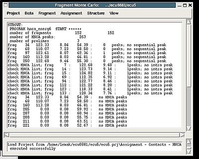
During the execution of this command the loaded HNCA peak list is validated. The validation results are shown in the project main window.
User have to check suspicious peaks going back to the spectra and correct the input peak list if it is needed.
Assignment>Contacts>NOE>fawn
:: Calculate fragment contact map CNOE_F.
Prerequisites:
♦ PB-fragments are loaded in memory;
♦ typing probabilities are calculated;
♦ N15-NOESY peak list is loaded in memory.
♦ tolerances are specified.
Results:
♦ contact map CNOE_F is calculated using N15-NOESY peak list and loaded in memory
Assignment>Contacts>NOE>abacus
:: Calculate both CNOE_B and CNOE_F contact maps.
Prerequisites:
♦ PB-fragments are loaded in memory
♦ typing probabilities are calculated
♦ N15-NOESY and C13-NOESY peak lists are loaded in memory
♦ tolerances are specified
Results:
♦ CNOE_F contact map is calculated using only N15_NOESY peak list
♦ CNOE_B contact map is calculated using both N15_NOESY and C13_NOESY peak lists that are interpreted by BACUS procedure
♦ Both calculated maps are loaded in memory
Assignment>Calculate Probabilities>SA
:: Calculate assignment probabilities
Prerequisites:
♦ protein sequence is loaded in memory
♦ PB-fragments are loaded in memory
♦ typing probabilities are calculated
♦ fragments contact map CHNCA is calculated
♦ at least one contact map CNOE_F or CNOE_B is calculated
Results:
♦ Assignment probability map PSA is calculated and loaded in memory.
Probabilistic mapping of PB fragments onto protein sequence is performed using Simulated Annealing (SA) Monte Carlo simulations.
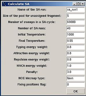
A new window “Calculate SA” is open were user can specify different parameters in the control file of the SA simulations (see Figure 2.9).
The main parameters to consider are:
<span />
- “Name of the SA run”. Normally the name is sa_run#. A new directory under this name will be created within PROJECTNAME/assign directory. SA calculations will be curried out and the results will be stored in this directory.
- “Size of the pool for unassigned fragments”. The number of positions that are appended to the protein sequence and discarded (unassigned) fragments, if there are any, will be located there. It is safe to over-estimate this number. (If this number is under-estimated, this will force the mapping of spurious spin-systems onto protein sequence);
- “Number of SA trajectories”. The time needed for calculations is proportional to this number. On the other hand, having more SA trajectories the assignment probabilities could be calculated more accurately. In the case of good data, when all SA trajectories converge to assignments with the same energy, 10-15 trajectories should be enough. In the case of poor data, it is better to calculate 40-50 SA trajectories.
- “NOE bbcmap type”. User should specify which one NOE contact map, (abacus) or (fawn) should be used in the calculations;
- “Fixing position flag”. If the flag is set to 1, sequence position of all fragments which has assignment ID > -99 will be fixed during the simulation.
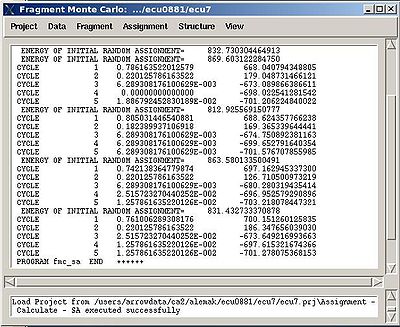
- “Final temperature”. Setting the optimal final temperature will provide all SA trajectories converge to optimal or sub-optimal assignments (the assignments that are in the vicinity of the global energy minimum). The optimal final temperature could be find by running one or a few SA runs with 3-4 trajectories and by analysing convergence of the trajectories from the report shown in the main FMCGUI window after each run (see Figure 2.10).
In the result of the SA calculations assignment probability map PSA is calculated and loaded in memory. The map is also saved in the file 'sa.probmap' located into PROJECTNAME/assignment/sa_run# directory.
Assignment>Calculate Probabilities>REM
:: Calculate assignment probabilities.
Prerequisites:
♦ protein sequence is loaded in memory
♦ PB fragments are loaded in memory
♦ typing probabilities are calculated
♦
fragments contact map CHNCA is calculated ♦ at least one contact map CNOE_F or CNOE_B is calculated
Results:
♦ assignment probbilities PREM are calculated and loaded in memory
Probabilistic mapping of PB fragments onto protein sequence is performed using Replica Exchange Method Monte Carlo simulations.
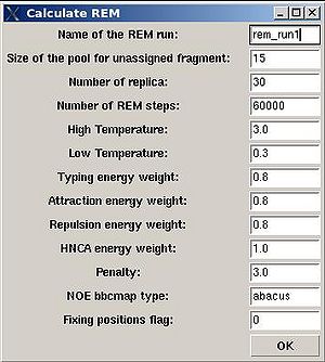
A new window “Calculate REM” is open were user can specify different parameters in the control file of the REM simulations (see Figure 2.11)
The main parameters to consider are:
- “Name of the REM run”. Normally the name is rem_run#. A new directory under this name will be created within PROJECTNAME/assign directory. REM calculations will be curried out and the results will be stored in this directory.
- “Size of the pool for unassigned fragments”. The number of positions that are appended to the protein sequence and discarded (unassigned) fragments, if there are any, will be located there. It is safe to over-estimate this number. (If this number is under-estimated, this will force the mapping of spurious spin-systems onto protein sequence);
- “Number of REM steps”. The time needed for calculations is proportional to this number. On the other hand, with more REM steps more extensive sampling of assignment space wil be achieved, which in turn results in more accurate assignment probabilities. This number should be increased for large proteins.
- “NOE bbcmap type”. User should specify which one NOE contact map, (abacus) or (fawn) should be used in the calculations;
- “Fixing position flag”. If the flag is set to 1, sequence position of all fragments which has assignment ID > -99 will be fixed during the simulation.
- “Low temperature”. The optimal low temperature will provide extensive sampling of should sub-optimal assignments during REM simulation.
User can check a correct setting of the low temperature as well as the number of REM steps by analysing a report shown in the main FMCGUI window after the calculations are done.
In the result, the 50 lowest energy assignments are used to calculate assignment probabilities . The probabilities PREM are loaded in memory and saved in the file ‘rem.prbmap’ located into PROJECTNAME/assign/rem_run# directory.
Assignment>Fix Assignment>Using Probability map
:: Perform sequence specific assignment of PB fragments using results of SA or REM calculations.
Prerequisites:
♦ protein sequence is loaded in memory;
♦ PB fragments loaded in memory;
♦ at least one SA or REM calculation of assignment probabilities is done
Results:
♦ Assignment ID for part (or all) of PB -fragments is specified
Calculation of assignment probabilities with FMCGUI could be repeated a few times using different methods and parameters. Results of each calculation are stored in a separate directory with the user-specified name. Therefore, there could be a few different directories (for example, sa_run1, sa_run2, rem_run0, rem_run1, rem_run2) located within PROJECTNAME/assign/ directory that contain different assignment probability maps.
User will be asked to select the calculation directory (sa_run# or rem_run#) and to specify the value of acceptance probability Pmin. Normally, Pmin =0.9 is appropriate. A fragment is considered to be assigned to a sequence position if the corresponding assignment probability (taken from the selected directory) is >= Pmin.
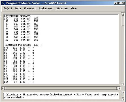
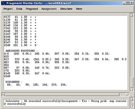
In the result, part of the PB-fragments will be assigned, namely, their assignment IDs A_id will be specified. The assignment report will be shown in the main FMCGUI window (see Figure 2.13) and saved in the corresponding simulation directory (‘sa.fix ‘or ‘rema.fix’ files) as well.
For each sequence position, the IDs of both unambiguously and ambiguously assigned fragments are shown in the report. The list of discarded fragments is also presented (see Figure 2.13).
Assignment>Fix Assignment>Manually
:: Fix sequence position of PB fragments manually
Prerequisites:
♦- protein sequence is loaded in memory;
♦- PB-fragments are loaded in memory;
Results:
♦ Assignment ID for selectedf PB fragments is specified
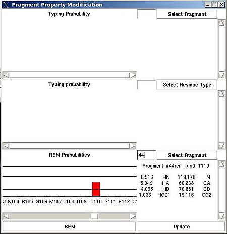
“Fragment Property Modification” (FPM) window will be open (see Figure 2.14). User can select a fragment in the bottom section of the window and the ingormation regarding the fragment assignemts will be displayed in this section. Namely, the graph shows assignment probabilities that are currently loaded in memory and the text part shows the chemical shifts making up the fragment and it’s assignment ID (A_id). Which assignment probabilities, PSA or PREM, are shown on the graph can be selectes by pressing left button at the bottom of FPM window.
To modify the current fragment assignment user have to select sequence position on the graph (using mouse right button) and then to press "Update" button. In the result, Assignment ID of the selected fragment will be set to the selected sequence position.
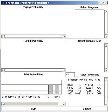
There are two special positions “U” and “B” shown on the graph at the end of the protein sequence (see Figure 2.15). Selecting “U” and pressing “Update” button results in changing assignment status of the fragments to Unassigned, that is A_id is set to -99. Selecting “B” and pressing “Update” button results in fixing fragment position in the pool of discarded fragments.
Assignment>Fix Assignment>Reset all
:: Change assignment status of all PB fragments to “Unassigned”.
Prerequisites:
♦ protein sequence is loaded in memory
♦ PB fragments are loaded in memory
Results:
♦ Assignment ID for all PB fragments is set to -99
Assignment>Load Probabilities
:: Load assignment probabilities
Prerequisites:
♦ protein sequence is loaded in memory;
♦ PB fragments are loaded in memory;
♦ SA or REM calculations of assignment probabilities are done
User have to select a directory where SA or REM calculations were done (sa_run# or rem_run#).
The assignment probabilities from the selected directory will be loaded in memory.
Structure>Constraints>Talos>calculate
:: Generate dihedral angle constraints.
Prerequisites:
♦ protein sequence is loaded in memory
♦ assigned shemical shifts are loaded in memory
Backbone dihedral angles are predicted using TALOS and then transformed to dihedral angle contraints.
In the result, the constraints are saved in two formats: files 'belok.aco' and 'prot_dihe.tbl' for CYANA and CNS calculations, respectively. Both files are saved in the project root directory.
Structure>Constraints>Talos>load
:: Load dihedral angle constraints in CYANA format (aco-file).
Structure>Constraints>H-bonds>Specify
:: Specify H-bond distance constraints manually.
Prerequisites:
♦ protein sequence is loaded in memory
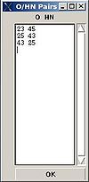
A new window “O/HN Pairs” is opened (see Figure ).
For each H-bond constraint, user have to specify O-HN pair by typing in the ID of residues corresponding to O and HN atoms. Pressing “OK” button will save H-Bond constraints on disk in two formats: files 'hbond.upl' and 'prot_hbond.tbl' for CYANA and CNS calculations, respectively. Both files are saved in the project root project directory.
Structure>Constraints>H-Bonds>load
:: Load HB-ond distance constraints in CYANA format (upl-file)
Structure>Calculate>Cyana
:: Set up new structure calculation run with CAYANA.
Prerequisites:
♦ protein sequence is loaded in memory
♦ assigned chemical shifts are loaded in memory
♦ N15-NOESY, C13-NOESY, and Arom-NOESY peak lists are loaded in memory
♦ specified tolerances
♦ dihedral angle constraints are created ( i.e. file “belok.aco” is present in the project root directory)
♦ Optional:
♦ HBond distance constraints (file “hbond.upl” is present in the project root directory)
♦ file that contains ZN ion ligands (file “zn_ligands” is present in the project root directory)
A new directory under the name that is specified by user (normally “crun#”) will be created inside project root directory PROJECTNAME. This directory contains all files required to start automatic structure calculations with CYANA.
Structure>Calculate>ABCUS
:: Sset up ABACUS structure calculations
Structure>RPF>RP
:: Perform Recall/Precision analysis of structural ensemble.
Prerequisites:
♦ protein sequence is loaded in memory
♦ assigned shemical shifts are loaded in memory
♦ N15-NOESY, C13-NOESY, and Arom-NOESY peak lists are loaded in memory
♦ specified tolerances
♦ coordinates of structural ensemble in CYANA format (final.pdb) or in CNS format
Results:
♦ summary report
♦ flase negative and false positive peak lists
The parameters to set up (see Figure ):
- “RP directory name”. Normally the name is rp#. A new directory under this name will be created within PROJECTNAME/assign directory. The results of the RPFanalysis will be stored in this directory.
- “sequence gap”. Residue pairs separated by less than the value of sequence gap will be excluded from generating expected peak lists.
- “cutting distance for recall”. Distance threshold for evaluating matching of an experimental peak to a structural ensemble (Recall score)
- “cutting distance for precition”. Distance threshold for generating expected peak from structural ensemble (Precision score)
The results of the RPF analysis will be saved in a new directory (for example, directory "rp1" on Figure) that is located in the project root directory. Results include peak lists in the SPARKY format of both false negative and false positive peaks for different NOESY spectra in a separate files.
Structure>RPF>DP
<div : To set up calculations of DP score with AutoStructure.</div>
Prerequisites:
- protein sequence is loaded in memory;
- assigned shemical shifts are loaded in memory;
- N15_NOESY, C13_NOESY, and Aron_NOESY peak lists are loaded in memory
- Specified tolerances.
- coordinates of structural ensemble in CYANA format (final.pdb) or in CNS format (prot_ref_al.pdb). pdb
Structure>Water refinement>calculate
: To set up water refinement of structural ensemble obtained with CYANA.
Prerequisites:
- structure calculation with CYANA should be done
Optional:
- RDC data in PALES format.
- file that contains ZN ion ligands (file “zn_ligands” )
User will be asked to specify the name of directory for water refinement calculations WATDIR and to select a number of files with coordinates and constraints. In addition to this user have to indicate cisProline residues (if there are any) and to specify protonation state of HIS residues which is double protonated by default (see Figure 2.18).
In the result, a new directory WATDIR will be created inside PROJECTNAME directory that contains all files and scripts required to carry out water refinement calculations with CNS. It is recommended to start calculations on linux cluster.
Structure>Water refinement>summary
: To create a summary.
Prerequisites:
- water refinement with CNS should be done.
User will be asked to specify residues used for structure superposition and to select the water refinement directory WATDIR (see figure 2.19).
The refined structural models will be superimpose and combined in one file. The created summary reports values of different energy components and constraint violation statistic for each structural model. A new directory WATDIR_results will be created. The directory contains final superimposed coordinates, distance and dihedral angle constrains in a format suitable for PDB deposition, summary and constraint violations report.
Structure>Add ZN ligands
: To create zn_ligands file.
User have to tipe in IDs of residues that ligate zinc ion into the popped up entry window “ZN ligands” (see Figure 2.20). If there are a few zinc ions, information for each ion should be provided in a separate row.
The file “zn_ligands” will be created inside the project root directory PROJECTNAME by pressing “OK” button.
Structure>RCI
<div : To calculate Random Coil Index.</div>
Random Coil Index is calculated using rci_v_1c.py script. New directory PROJECTNAME/rci that contains the results of calculations is created.
This section provides means to visualize data and calculation results.
View>Fragment
: To display current fragment properties.
This command opens “Fragment Graph” (FG) window were all properties of a selected fragment that currently are loaded in memory will be displayed (see Figure 2.21).
The chemical shifts making up the fragment are shown in the middle part of the window. The heading line (for example, line “Fragment #21 rem_run1 L108” shown on Figure 2.21) shows fragment ID (#21), the name of directory that contains assignment probabilities used to assign the fragment (rem_run1) and sequence position to which the fragment is assigned (L108). All other fragment properties are shown in the form of graphs. Typing probabilities the top section of the window one can see typing probabilities and both assignment probabilities and are shown on three graph on the top part of the FG window. It is also indicated the name of the directories from which the displayed assignment probabilities were loaded. Two graphs on the bottom part of the FG window shows a column ( or ) and a row ( or ) of a contact map calculated from NOESY data, respectively. Here U_id is selected fragment ID, while f is any fragment ID for which the corresponding score is > 0. What contact map, or ), is shown on the graphs is indicated on the bar at the bottom of FG window. Clicking on this bar by mouse will switch from one contact map to another.
The contact map is shown on this graph implicitly as well by color of graph bars.
For example, on the Figure 2.21 the elements of contact map related to the fragment 21 are shown. The score for fragment 21 to be before the fragments 37, 20 and 17 in protein sequence are shown in magenta which means that these connections being derived from NOESY data are supported by HNCA spectra as well. The score for fragment 21 to be before the fragments 22 and 4 are shown in red meaning that theses connections are not supported by HNCA spectra.
View>Assignment
<div : To display assignment results.</div>
The user is asked to select a directory were assignment probabilities were calculated
(sa_run# or rem_run#).
New “Assignments Graphs” (AG) window pops up (see figure 2.22). This window provides user with graphical means to manipulate PB-fragment’s assignments without making changes of assignment status of PB-fragments in memory. The current fragment’s assignment, taken from the memory, altogether with different scores associated with this assignment is shown when AG window is opened. The fragments that currently are not assigned are also shown in the bottom-right part of the AG window. User can modify the current assignment and to observe the resulting changes in the scores.
A particular fragment’s assignment is displayed on the left part of the AG window. The graph at the bottom shows ID of fragments assigned to each sequence position, while four graphs on the top show different scores that correspond to this assignment, namely, HNCA score, NOE scores, typing and assignment probabilities that currently loaded in memory. The scroll bar at the bottom allows user to move along protein sequence.
In order to modify the assignment user have first to select protein sequence segment of interest by clicking on IDs of two residues that correspond to the edges of the segment. The colour of these residues, for example K56 and D59, will change to red (see Figure 2.23). Then pressing on “Select Segment” bar at the bottom of AG window will result in possible assignment for the selected window to be shown on top-right corner of AG window. The possible assignments for the selected sequence segment are taken form the selected directory shown on the title bar and correspond to sub-optimal fragment assignments sampled during SA or REM calculations
The new assignment for the sequence segment should be selected from the list of possible assignments using mouse. The color of the selected line will turn red (see Figure 2.23). In the case user want to consider an assignment that is not present in the list, he should select any assignment from the list ant modify it by pressing the button “Edit” at the bottom of the AG window. A new window “Edit Assignment” pops up, and user can modify the assignment by typing changes in this window see Figure 2.24).
Once a new assignment for the sequence segment is selected the current fragments assignment shown on the left part of AG window can be modified by pressing button “Update” (see Figure 2.25)
