Routine Processing Procedure for 3D 15N and 13C-edited Experiments
Jump to navigation
Jump to search
NMR Data Processing > Routine 3D Experiments via NMRPipe
Brief Description
The procedure for processing a 3D dataset is fairly similar to the ones described for the 2D dataset along with additional parameters for a third dimension (generally refered to as the z dimension). For nD dataset where the indirect dimension(s) is collected with few points, it is often advantageous to increase the number of points and digital resolution using ‘Linear Prediction’. This calculation determines the frequency and decay rate of the peaks in an FID or interferrogram, and extends them mathematically. It is very useful for 15N and 13C-edited 3D dataset where experimental time is needed to improve S/N, so the number of increments is limited. It is important to mention that ‘Linear Prediction’ on the selected dimension of a 3D dataset is performed after the other two dimensions have been processed. An example processing script for HNCO experiment is shown here, where the HN dimension (x) and N dimension (z) are first processed followed by the linear prediction and processing of the CO dimension (y). The N dimension is then inverse transformed, linear predicted, and retransformed. This processing script is also applicable to the majority of 3D 15N and 13C-edited datasets for protein related work.
Software Information
NMRPipe (download information and user manual)
Brief descriptions of specific functions are accessible via nmrPipe –
‘nmrPipe –help’ will list most functions.
‘nmrPipe –fn GM –help’ will give description of the GM function.
Supported Platforms
Linux (RedHat Linux/Fedora)
Mac OS X (10.3.4 and up)
SGI Irix (6.2 and up)
Sparc Solaris (2 and up)
Windows XP Pro with Microsoft Services for UNIX (SFU 3.5).
Converting Spectrometer Data into NMRPipe Format
The conversion of data from spectrometer format to NMRPipe format is usually done using a build-in program called ‘varian’ for Varian a dataset ('bruker' for a Bruker dataset and 'delta' for dataset from JEOL). Brief summaries of the build-in program can be found here.
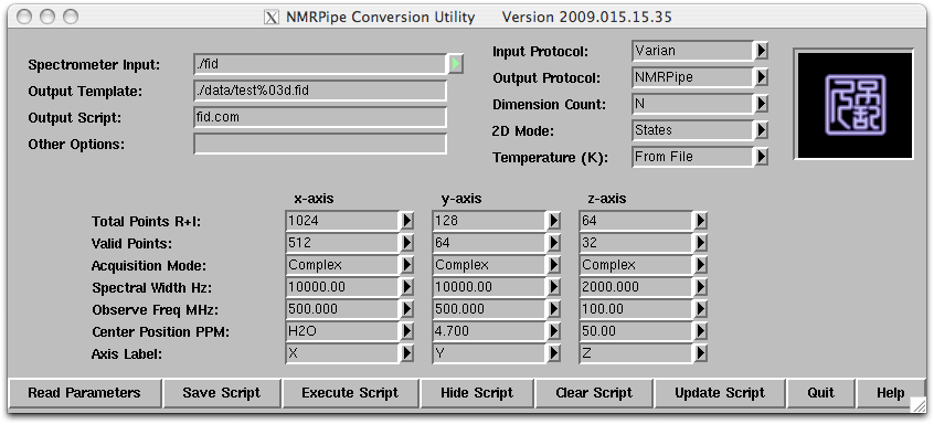
Step 1: Under the same directory where the procpar and fid files are, type ‘varian’ and this will start a tcl/tk script that brings up two windows.
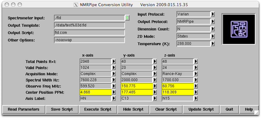
Step 2: Click on the ‘Read Parameters’ button and the script will read the parameter file (‘procpar’) and update the parameters.
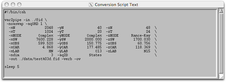
The template shows parameters for three dimensions x, y, and z for HN, CO, and N, respectively. More detailed description of the input script can be found at routine 2D experiment or NMRPipe user manual.
‘-aqORD 1’ !!! Varian dataset when ‘array=phase,phase2’
‘-xMODE complex’ !!! For the direct dimension
‘-yMODE: complex’ !!! For the CO dimension
‘-zMODE: Rance-Kay’ !!! For sensitivity enhanced experiment
Step 3: Click on ‘Save Script’, and then ‘Execute Script’. The converted planes in NMRPipe format will be stored in the ‘data’ directory along with an UNIX shell script called ‘fid.com’.
Processing and Visualizing 3D Dataset
For information on the macro editor of nmrDraw, see routine processing procedure for 2D experiment. An example of processing script for a 3D HNCO spectrum with linear prediction in the y and z dimensions is shown below.
!!! Part 1, process the directly-detected x-axis !!!
xyz2pipe -in fid/test%03d.fid -x -verb \
| nmrPipe -fn SOL \ ## Removed residual solvent
| nmrPipe -fn SP -off 0.5 -end 0.98 -pow 2 -c 0.5 \ ## Apodization
| nmrPipe -fn ZF -auto \ ## Zero fill
| nmrPipe -fn FT \ ## Fourier transformation
| nmrPipe -fn PS -p0 43 -p1 0.0 -di \ ## Phase correction
| nmrPipe -fn EXT -left -sw \ ## Extract left half spectrum
| pipe2xyz -out lp/test%03d.ft3 -x
!!! Part 2, process the indirectly-detected z-axis !!!
xyz2pipe -in lp/test%03d.ft3 -z -verb \
| nmrPipe -fn SP -off 0.5 -end 0.95 -pow 1 -c 0.5 \ ## Apodization
| nmrPipe -fn ZF -auto \ ## Zero fill
| nmrPipe -fn FT \ ## Fourier transformation
| nmrPipe -fn PS -p0 0.0 -p1 0.0 -di \ ## Phase correction
| pipe2xyz -out lp/test%03d.ft3 -z –inPlace
!!! predict and process the indirect-detected y-axis !!!
xyz2pipe -in lp/test%03d.ft3 -y -verb \
| nmrPipe -fn LP -fb -ord 10 \ ## Linear Prediction
| nmrPipe -fn SP -off 0.5 -end 0.98 -pow 1 -c 1.0 \ ## Apodization
| nmrPipe -fn ZF -auto \ ## Zero fill
| nmrPipe -fn FT \ ## Fourier transformation
| nmrPipe -fn PS -p0 -135 -p1 180 -di \ # Phase correction
| pipe2xyz -out lp/test%03d.ft3 -y -inPlace
!!! inverse, predict, and re-process the z-axis
xyz2pipe -in lp/test%03d.ft3 -z -verb \
| nmrPipe -fn HT -auto \
| nmrPipe -fn PS -inv -hdr \
| nmrPipe -fn FT -inv \
| nmrPipe -fn ZF -inv \
| nmrPipe -fn SP -inv -hdr \
| nmrPipe -fn LP -fb \ ## Linear prediction
| nmrPipe -fn SP -off 0.5 -end 0.98 -pow 1 -c 0.5 \ ## Apodization
| nmrPipe -fn ZF -auto \ ## Zero fill
| nmrPipe -fn FT \ ## Fourier transformation
| nmrPipe -fn PS -hdr -di \
| pipe2xyz -out lp/test%03d.ft3 -z -inPlace
Suggested Workflow
Step 1: Generate the processing script with the appropriate commands and functions using the macro editor or modified existing script. Set both the p0 and p1 phasing values of the direct dimension to 0.
Step 2: Execute the processing script in a UNIX terminal. The 2D projection planes of the 3D dataset can be created using the build-in program readROI for phase correction (execute the following command in a UNIX terminal, ‘nmrWish –f Project.txt’). Load the projection plane into nmrDraw to perform phase correction and optimize the applied functions. A 1D horizontal trace can be activate by typing ‘h’ in the spectrum window and the phase of the dimension can be adjusted using the P0 and P1 slider bars. To phase an indirect dimension, type 'v'. Now the P0 and P1 slider bars will change the phase of the indirectly detected dimension.
Step 3: Execute the processing script with optimized parameters.
Step 4: Convert the processed data to the format of graphical NMR assignment program.


