Measuring 15N T1 and T2 relaxation times (Varian)
Correlation Time and NMR Measurement Time Prediction
Experimental Setup
Run the HTP_t1t2_setup script to setup the following experiments:
- 2D [15N, 1H] HSQC, ~1.5h for SN analysis
- NHonly='n' C13refoc='y' ni=256 f1180='n' phase=1,2 nt=8 ss=32
- 1D 15N T1, ~30 min
- ni=1 phase=1 T1='y' f1180='n' NHonly='n' C13refoc='n' ss=256 nt=128
- relaxT=0.1, 0.2, 0.3, 0.4, 0.7, 1.0, 1.5, 2.0
- 1D 15N T2, ~30 min
- ni=1 phase=1 T2='y' f1180='n' NHonly='n' C13refoc='n' ss=256 nt=128
- relaxT=0.01,0.03,0.05,0.07,0.09,0.11,0.13,0.15,0.17 maxrelaxT=0.17
Key issues:
- For most proteins it is recommended to run T1 and T2 experiments for at least 30 min each to achieve adequate S/N on a room-temperature probe. Short measurement times may lead to underestimated tc values. With cryogenic probes or very concentrated (> 1 mM) samples the minimum measurement time may be smaller.
- Short d1 delays (~1 s) may lead to incorrect integral for the first T1 point. However, long d1 values may lead to a large residual water line and non-uniform baseline, especially on a cryoprobe. See what works best for the particular sample and spectrometer.
- relaxT must be given as a multiple of 10 ms for T1 and odd multiple of 10 ms for T2.
- maxrelaxT is not used in T1 measurements.
- Avoid sampling T2 points beyond 250 ms - it may cause excessive sample heating.
- Intermediate tc values (between monomer and dimer) may indicate transient dimerization. Dilution studies are then required.
- The tc value is calculated under assumption of isotropic tumbling. For example, if a protein consists of long parallel a-helices the reported tc will indicate a larger molecular weight.
Correlation Time Measurement
Based on the Stokes's law, the isotropic rotational correlation time for approximately spherical globular proteins is a function of the effective hydrodynamic radius of the protein, which provides a simple way to check the oligomerizaiton status of protein in solution. Here is the basic law: the correlation time in nanoseconds is approximately half of the value of the protein's molecular weight in kilodaltons.
A protein's rotational correlation time (Tauc) can be quickly estimated from average 15N T1 and T2 relaxation times.
To calculate Tauc:
- Process the data in Buffalo.VNMR with wft and adjust the phase for pure absorption.
- Invoke dc to correct baseline shift and slope. You can expand the spectrum for better results.
- Invoke dscale and setref to make sure the ppm scale is correct - required for the tc macro.
- Display all spectra with dssh and check that
- baseline is flat and uniform across points.
- Spectral intensity follows an exponential decay.
- Run tc([T1exp, T2exp, [ppm1, ppm2]]), where the first two arguments are T1 and T2 experiment numbers, and the last two optional arguments specify the integration range in ppm. By default, integration is performed over the range between 10.5 ppm and 8.5 ppm to exclude signals from side-chain CONH2 groups (6 - 7 ppm) and unfolded parts (8 ppm).
Tc macro
The tc macro is invoked by typing tc([T1exp, T2exp, [ppm1, ppm2]]) at the VNMR prompt. T1exp and T2exp are the experiment numbers of T1 and T2 experiments, respectively. As an option, the integration range in ppm can be specified with the third and fourth arguments. The default integration range is chosen between 10.5 and 8.5 ppm to avoid the resonances from side chain -CONH2 groups and backbone amides from unfolded regions. If called with no arguments tc will prompt for experiment numbers and use the default integration range.
Tc macro requires t1a, t2a and intav macros. The intav macro performs integration stores the integral values in the fp.out file. t1a and t2a macros extract T1 and T2 relaxation times from the exponential fitting to the data in fp.out. Manual phase and drift correction (dc) of 1D spectra should be performed first to get accurate results.
τ_c is then calculated as
τ_c = sqrt(6 * (T1 / T2) - 7) / (2 ω(N)),
where ω(N) is the 15N frequency. This formula is derived from equation (8) in Kay, Torchia and Bax, Biochemistry 1989, 28, p8972-8979 by keeping only J(0) and J(ω(N)) terms and neglecting all higher frequencies. The complete equation (8) cannot be solved analytically for τ_c, and the simplified formula presented here should yield accurate results for systems with τ_c >> 0.5 ns.
The reported error range is from simple error propagation of the exponential fit error and is rather crude. Strictly speaking, such simple error propagation does not apply here, because the expected error distribution for τ_c is asymmetric.
To install tc macro:
- Download tc_macro.tar into the user maclib directory (~/vnmrsys/maclib/)
- Unpack it with tar xvf tc_macro.tar
Measurement Time Prediction
The minimum measurement time of (4,3)D GFT experiments can be reliably predicted from the S/N distribution of a 2D [15N, 1H] HSQC and the rotational correlation time tau_c. First, you need to generate an integrated peaklist.
Peak Integration in 2D [15N, 1H] HSQC
Having processed 2D (15N, 1H) HSQC as described in data process, one can do the peak picking and integration of 2D (15N, 1H) HSQC manualy or semi-automaticlly as following:
- Peak picking and integration by using program XEASY
- Use command ns to load the spectrum
- Use ls to load the corresponding sequence file (optional)
- Use in to automatic pick peaks with total peak number slightly more than expected by select adjust contour level; then manually remove side-chain amide peaks
- Use mn to measure noise level, and use tw to display the noise level value. Normally the value of 2.5 times of standard deviation ( ~250 if the noise level has been normalized ) is taken as noise level.
- Use ip to choose peak height (m) as integration mode, and use "ii" to integrate the whole spectrum. An XEASY external program "PeakintI" can be used to obtain more accurate peak height values, which is discribed below.
- Use wp to save the peak list.
- More accurate peak height measurement by using program PeakintI.
Type command:
peakintI ../data/NHsqc6001 nhsqcsa_b.peaks 250 -i -t 2 2 0.1
where the nhsqcsa_b.peaks is the input peak list and the output file will be inhsqcsa_b.peaks. - Combing atom name informaiton in the peak list for S/N distribution (optional).
S/N distribution analysis for 2D (15N, 1H) HSQC
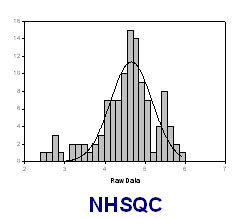
The SN distribution of resonances in a NMR spectra can be fit to the Gaussian distribution:
f= a*exp(-0.5*((ln(SN_i)-ln(SN_0))/b)^2)
where SN_0 is the most populated S/N observed, f is the expected population at a certern SN value SN_i, a and b are contants.
The SN of NHSQC SN_0 can be obtained as following:
- Calculate ln(SN) for each peak from the peak height and noise level, e.g. by using EXCEL
- Obtain SN distribution (population v.s. ls(SN)) by using Sigma-Plot
- By using Sigma-Plot, fitting SN distribution to Gaussian distribution and obtain SN_0, constant a and b.
Calculation of Measurement Time
The SN distribution of resonances in other NMR spectra can also be fit to the Gaussian distribution as in 2D (15N, 1H) NHSQC:
f= a*exp(-0.5*((ln(SN_i)-ln(SN_0))/b)^2)
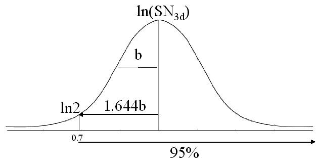
where SN_0 is the most populated SN observed, f is the expected population at a certain SN value SN_i, a and b are constants. Based on this equation, one can calculate the expected SN_0 for a required peak detection yield.
Assuming that a peak shall have at least SN value of 2 in order to be observed or detected, and the average b for (4,3) GFT experiments is 0.8; if 95% peak detection yield is required, the exptected SN_0 is:
SN_0=exp(ln2+1.644*b)=7.4
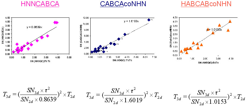
NMR measurement time of (4,3) GFT HNNCABCA, (4,3)D GFT CABCAcoNHN and (4,3)D HABCABCONHN can be calculated from the following equation:
T_43d= ((SN_43d* Tauc^2)/(SN_2d*A))^2
where T_43d is the required time for (4,3) GFT experiment, SN_43d is the expected SN value of (4,3)D GFT experiments, SN_2d is the SN per hour of 2D (15N, 1H) HSQC. =A= is constant, which has value of 0.8639 for (4,3) GFT HNNCABCA, 1.6019 for (4,3)D GFT CABCAcoNHN and 1.0153 for (4,3)D HABCABCONHN.
One can use UBNMR to run the measurement time predition by the following command:
predict T2d SN2d Tc
where
- T2d is the acquisition time of 2D [15N,1H] HSQC in hours
- SN2d is the SN distribution average of 2D [15N,1H] HSQC
- Tc is the rotational correlation time of protein in nanoseconds.
-- AlexEletski - 03 Mar 2008


