Estimation of measurement time: Difference between revisions
(Created page with 'The minimum measurement time of (4,3)D GFT experiments can be reliably predicted from the S/N distribution of a 2D [15N, 1H] HSQC and the rotational correlation time tau_c. First…') |
No edit summary |
||
| Line 1: | Line 1: | ||
The minimum measurement time of (4,3)D GFT experiments can be reliably predicted from the S/N distribution of a 2D [15N, 1H] HSQC and the rotational correlation time tau_c. First, you need to generate an integrated peaklist. | The minimum measurement time of (4,3)D GFT experiments can be reliably predicted from the S/N distribution of a 2D [15N, 1H] HSQC and the rotational correlation time tau_c. First, you need to generate an integrated peaklist. | ||
==== '''Peak Integration in 2D [15N, 1H] HSQC''' ==== | ==== '''Peak Integration in 2D [15N, 1H] HSQC''' ==== | ||
Having processed 2D (15N, 1H) HSQC as described in data process, one can do the peak picking and integration of 2D (15N, 1H) HSQC | Having processed 2D (15N, 1H) HSQC as described in data process, one can do the peak picking and integration of 2D (15N, 1H) HSQC manually or semi-automatically as following: | ||
*Peak picking and integration by using program XEASY | *Peak picking and integration by using program XEASY | ||
| Line 11: | Line 11: | ||
##Use <tt>in</tt> to automatic pick peaks with total peak number slightly more than expected by select adjust contour level; then manually remove side-chain amide peaks | ##Use <tt>in</tt> to automatic pick peaks with total peak number slightly more than expected by select adjust contour level; then manually remove side-chain amide peaks | ||
##Use <tt>mn</tt> to measure noise level, and use <tt>tw</tt> to display the noise level value. Normally the value of 2.5 times of standard deviation ( ~250 if the noise level has been normalized ) is taken as noise level. | ##Use <tt>mn</tt> to measure noise level, and use <tt>tw</tt> to display the noise level value. Normally the value of 2.5 times of standard deviation ( ~250 if the noise level has been normalized ) is taken as noise level. | ||
##Use <tt>ip</tt> to choose peak height (m) as integration mode, and use "ii" to integrate the whole spectrum. An [[NESG:XEASY|XEASY]] external program "PeakintI" can be used to obtain more accurate peak height values, which is | ##Use <tt>ip</tt> to choose peak height (m) as integration mode, and use "ii" to integrate the whole spectrum. An [[NESG:XEASY|XEASY]] external program "PeakintI" can be used to obtain more accurate peak height values, which is described below. | ||
##Use <tt>wp</tt> to save the peak list. | ##Use <tt>wp</tt> to save the peak list. | ||
| Line 23: | Line 23: | ||
The SN distribution of resonances in a NMR spectra can be fit to the Gaussian distribution: | The SN distribution of resonances in a NMR spectra can be fit to the Gaussian distribution: | ||
[[Image: | [[Image:Sn nhsqc.jpg]] | ||
<br><tt>f= a*exp(-0.5*((ln(SN_i)-ln(SN_0))/b)^2) </tt><br> where <tt>SN_0</tt> is the most populated S/N observed, <tt>f is the expected population at a | <br><tt>f= a*exp(-0.5*((ln(SN_i)-ln(SN_0))/b)^2) </tt><br> where <tt>SN_0</tt> is the most populated S/N observed, <tt>f is the expected population at a certain SN value SN_i</tt>, <tt>a and b</tt> are constants. | ||
The SN of NHSQC <tt>SN_0</tt> can be obtained as following: | The SN of NHSQC <tt>SN_0</tt> can be obtained as following: | ||
| Line 37: | Line 37: | ||
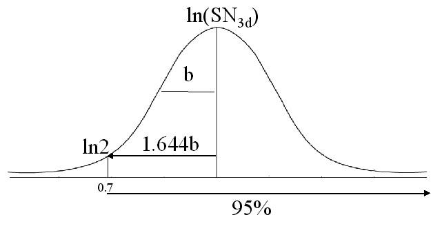
The SN distribution of resonances in other NMR spectra can also be fit to the Gaussian distribution as in 2D (15N, 1H) NHSQC:<br><br> <tt>f= a*exp(-0.5*((ln(SN_i)-ln(SN_0))/b)^2)</tt> <br><br> where <tt>SN_0</tt> is the most populated SN observed, <tt>f</tt> is the expected population at a certain SN value <tt>SN_i</tt>, <tt>a</tt> and <tt>b</tt> are constants. Based on this equation, one can calculate the expected SN_0 for a required peak detection yield. | The SN distribution of resonances in other NMR spectra can also be fit to the Gaussian distribution as in 2D (15N, 1H) NHSQC:<br><br> <tt>f= a*exp(-0.5*((ln(SN_i)-ln(SN_0))/b)^2)</tt> <br><br> where <tt>SN_0</tt> is the most populated SN observed, <tt>f</tt> is the expected population at a certain SN value <tt>SN_i</tt>, <tt>a</tt> and <tt>b</tt> are constants. Based on this equation, one can calculate the expected SN_0 for a required peak detection yield. | ||
Assuming that a peak shall have at least SN value of 2 in order to be observed or detected, and the average b for (4,3) GFT experiments is 0.8; if 95% peak detection yield is required, the | Assuming that a peak shall have at least SN value of 2 in order to be observed or detected, and the average b for (4,3) GFT experiments is 0.8; if 95% peak detection yield is required, the expected SN_0 is:<br><br><tt>SN_0=exp(ln2+1.644*b)=7.4 </tt><br><br> | ||
[[Image:Sn2.jpg]] | [[Image:Sn2.jpg]] | ||
| Line 45: | Line 45: | ||
[[Image:Sn3.jpg]] | [[Image:Sn3.jpg]] | ||
One can use [[NESG:UBNMR|UBNMR]] to run the measurement time | One can use [[NESG:UBNMR|UBNMR]] to run the measurement time prediction by the following command: <br><br><br> <tt>predict T2d SN2d Tc</tt><br>where | ||
*<tt>T2d</tt> is the acquisition time of 2D [15N,1H] HSQC in hours | *<tt>T2d</tt> is the acquisition time of 2D [15N,1H] HSQC in hours | ||
Latest revision as of 15:47, 15 December 2009
The minimum measurement time of (4,3)D GFT experiments can be reliably predicted from the S/N distribution of a 2D [15N, 1H] HSQC and the rotational correlation time tau_c. First, you need to generate an integrated peaklist.
Peak Integration in 2D [15N, 1H] HSQC
Having processed 2D (15N, 1H) HSQC as described in data process, one can do the peak picking and integration of 2D (15N, 1H) HSQC manually or semi-automatically as following:
- Peak picking and integration by using program XEASY
- Use command ns to load the spectrum
- Use ls to load the corresponding sequence file (optional)
- Use in to automatic pick peaks with total peak number slightly more than expected by select adjust contour level; then manually remove side-chain amide peaks
- Use mn to measure noise level, and use tw to display the noise level value. Normally the value of 2.5 times of standard deviation ( ~250 if the noise level has been normalized ) is taken as noise level.
- Use ip to choose peak height (m) as integration mode, and use "ii" to integrate the whole spectrum. An XEASY external program "PeakintI" can be used to obtain more accurate peak height values, which is described below.
- Use wp to save the peak list.
- More accurate peak height measurement by using program PeakintI.
Type command:
peakintI ../data/NHsqc6001 nhsqcsa_b.peaks 250 -i -t 2 2 0.1
where the nhsqcsa_b.peaks is the input peak list and the output file will be inhsqcsa_b.peaks. - Combing atom name informaiton in the peak list for S/N distribution (optional).
S/N distribution analysis for 2D (15N, 1H) HSQC
The SN distribution of resonances in a NMR spectra can be fit to the Gaussian distribution:
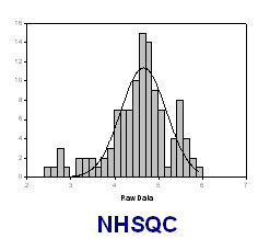

f= a*exp(-0.5*((ln(SN_i)-ln(SN_0))/b)^2)
where SN_0 is the most populated S/N observed, f is the expected population at a certain SN value SN_i, a and b are constants.
The SN of NHSQC SN_0 can be obtained as following:
- Calculate ln(SN) for each peak from the peak height and noise level, e.g. by using EXCEL
- Obtain SN distribution (population v.s. ls(SN)) by using Sigma-Plot
- By using Sigma-Plot, fitting SN distribution to Gaussian distribution and obtain SN_0, constant a and b.
Calculation of Measurement Time
The SN distribution of resonances in other NMR spectra can also be fit to the Gaussian distribution as in 2D (15N, 1H) NHSQC:
f= a*exp(-0.5*((ln(SN_i)-ln(SN_0))/b)^2)
where SN_0 is the most populated SN observed, f is the expected population at a certain SN value SN_i, a and b are constants. Based on this equation, one can calculate the expected SN_0 for a required peak detection yield.
Assuming that a peak shall have at least SN value of 2 in order to be observed or detected, and the average b for (4,3) GFT experiments is 0.8; if 95% peak detection yield is required, the expected SN_0 is:
SN_0=exp(ln2+1.644*b)=7.4

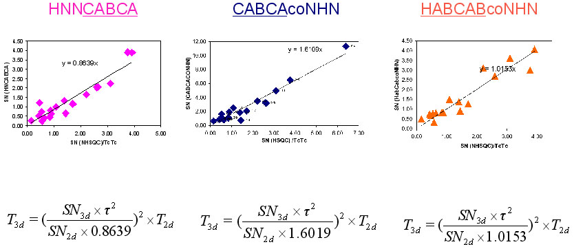
NMR measurement time of (4,3) GFT HNNCABCA, (4,3)D GFT CABCAcoNHN and (4,3)D HABCABCONHN can be calculated from the following equation:
T_43d= ((SN_43d* Tauc^2)/(SN_2d*A))^2
where T_43d is the required time for (4,3) GFT experiment, SN_43d is the expected SN value of (4,3)D GFT experiments, SN_2d is the SN per hour of 2D (15N, 1H) HSQC. =A= is constant, which has value of 0.8639 for (4,3) GFT HNNCABCA, 1.6019 for (4,3)D GFT CABCAcoNHN and 1.0153 for (4,3)D HABCABCONHN.

One can use UBNMR to run the measurement time prediction by the following command:
predict T2d SN2d Tc
where
- T2d is the acquisition time of 2D [15N,1H] HSQC in hours
- SN2d is the SN distribution average of 2D [15N,1H] HSQC
- Tc is the rotational correlation time of protein in nanoseconds.
-- AlexEletski - 03 Mar 2008