HA and HB Assignment with GFT in XEASY: Difference between revisions
Jump to navigation
Jump to search
No edit summary |
No edit summary |
||
| Line 9: | Line 9: | ||
#Go to the directory <tt>/analisys/xeasy/habcab</tt> and copy the <tt>final-clean.seq</tt> and <tt>final-clean.prot</tt> files from the backbone directory | #Go to the directory <tt>/analisys/xeasy/habcab</tt> and copy the <tt>final-clean.seq</tt> and <tt>final-clean.prot</tt> files from the backbone directory | ||
#Run <tt>makeHabcabPeaks</tt> in [[UBNMR|UBNMR]] to generate an extended [[XEASY Atom List|AtomList]] <tt>habcabconhI1.prot</tt> (containing linear combinations of 13CAB and 1HAB shifts) and the initial HABCAB [[XEASY Peak List|PeakList]] <tt>habcabconhI1.peaks</tt> to guide manual peak identification in (4,3)D HABCAB(CO)NHN. Peaks are colored according to type of sub-spectrum and type of proton involved in the GFT dimension. | #Run <tt>makeHabcabPeaks</tt> in [[UBNMR|UBNMR]] to generate an extended [[XEASY Atom List|AtomList]] <tt>habcabconhI1.prot</tt> (containing linear combinations of 13CAB and 1HAB shifts) and the initial HABCAB [[XEASY Peak List|PeakList]] <tt>habcabconhI1.peaks</tt> to guide manual peak identification in (4,3)D HABCAB(CO)NHN. Peaks are colored according to type of sub-spectrum and type of proton involved in the GFT dimension. | ||
#In XEASY | #In XEASY | ||
##use <tt>ns</tt>, <tt> | ##use <tt>ns</tt> to load '''subspectrum I''', <tt>HABCABcoNH1</tt>, from <tt>/protName/analysis/xeasy/habcab/</tt> | ||
# | ##<tt>cp</tt> to display the spectrum as a contour plot | ||
# | ##<tt>ls</tt> to load the [[XEASY Sequence List|SequencList]] (<tt>protein.seq</tt>) | ||
##<tt>lc</tt> to load [[XEASY Atom List|AtomList]] (<tt>habcabconhI1.prot</tt>) | |||
# | ##<tt>lp</tt> to load the starting [[XEASY Peak List|PeakList]] (<tt>habcabconhI1.peaks</tt>) | ||
# | ##<tt>se</tt> to create the strips for '''subspectrum I''' | ||
# | ##<tt>ns</tt> to load '''subspectrum II''', <tt>HABCABcoNH2</tt> | ||
##<tt>cp</tt> to display the spectrum as a contour plot | |||
##<tt>se</tt> to create the strips for '''subspectrum II''' and <tt>gs</tt> to display the strips (see Figure 1, below) | |||
##<tt>pw</tt> and click the box for '''assignment y''' to display the assignments in the GFT HabCab dimension | |||
##<tt>mr</tt> to accurately position the peaks along w1(13C) and <tt>bs</tt> / <tt>fs</tt> to move through the strips | |||
###when moving peaks, be sure to move the proper peak for each of the subspectra ('''NOTE''': if the spectra were processed using Buffalo's PERL scripts, then '''subspectrum I''' should use the "plus" peaks -- CA+HA, CB+HB2, CB+HB3, etc.) | |||
###if the HA1/2 or HB2/3 peaks are degenerate, move both of the peak markers to the same position and try to resolve them in the NOESY<br> | |||
###for non-degenerate HB2/3 (or HA1/2) peaks, place the CB+HB3 and CB-HB3 peaks on the "outside" and the CB+HB2 and CB-HB2 peaks on the "inside" of the peak pairs | |||
###if you are unable to correctly identify the peak pairs (e.g., CA+HA and CA-HA), use the 13C single-quantum chemical shifts from the backbone experiments to identify the center of the peak pair | |||
#In UBNMR, run <tt>updateHabAtom</tt> to update single-quantum 1HAB and 13CAB shifts as <tt>habcabconhO2.prot</tt>. A least-squares fit provides the single-quantum HA/HB chemical shifts (consistency of peaks representing different linear combinations of shifts is checked by UBNMR in oder to identify inadvertently 'mis-picked' peaks; a warning is then provided). | #In UBNMR, run <tt>updateHabAtom</tt> to update single-quantum 1HAB and 13CAB shifts as <tt>habcabconhO2.prot</tt>. A least-squares fit provides the single-quantum HA/HB chemical shifts (consistency of peaks representing different linear combinations of shifts is checked by UBNMR in oder to identify inadvertently 'mis-picked' peaks; a warning is then provided). | ||
#In XEASY, double-check the peak positions for residues that gaving large error. Repeat previous step and this step till no improvement can be made. | #In XEASY, double-check the peak positions for residues that gaving large error. Repeat previous step and this step till no improvement can be made. | ||
#Now it is ready to move to [[XEASY Side Chain Assignments|Side Chain Assignments]] | #Now it is ready to move to [[XEASY Side Chain Assignments|Side Chain Assignments]] | ||
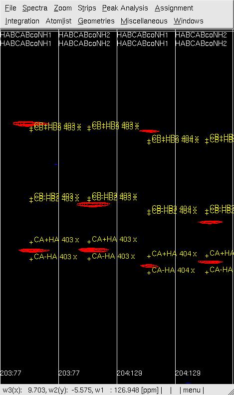
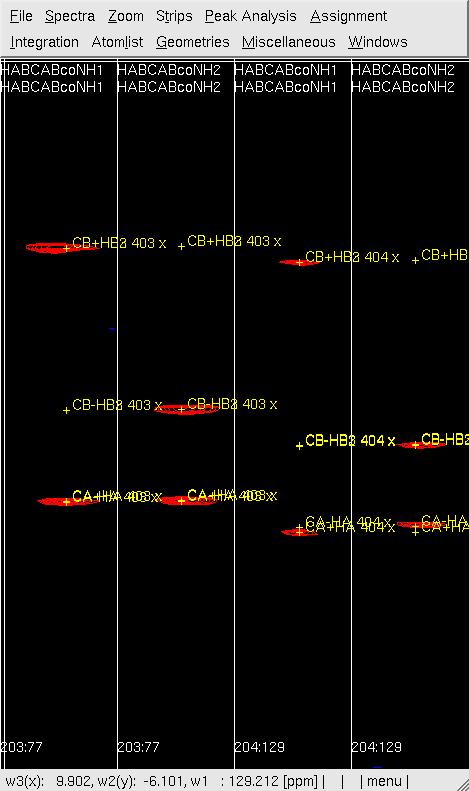
#'''Figure 1: Example of (4,3)D GFT HABCAB(CO)NHN analysis before (left) and after (right) peak position adjustment by <tt>mr</tt>.''' <br> [[Image:XEASY hab5.jpg]] [[Image:XEASY hab4.jpg]] <br> | |||
<br> | <br> | ||
Latest revision as of 18:07, 1 December 2009
HA And HB Assignments with XEASY/UBNMR
HA and HB assignments provide the bridge from Backbone Assignment to the complete Side Chain Assignments.
Analysis of the(4,3)D GFT HABCAB(CO)NHN
The sequence-specific 15N / 1HN / 13CAB resonance assignments obtained as described in backbone assignment are first used to also obtain 1HA and 1HB shift assignments by analyzing (4,3)D HABCAB(CO)NHN. Then, shifts of more peripheral aliphatic spins are obtained from (4,3)D HCCH.
- Go to the directory /analisys/xeasy/habcab and copy the final-clean.seq and final-clean.prot files from the backbone directory
- Run makeHabcabPeaks in UBNMR to generate an extended AtomList habcabconhI1.prot (containing linear combinations of 13CAB and 1HAB shifts) and the initial HABCAB PeakList habcabconhI1.peaks to guide manual peak identification in (4,3)D HABCAB(CO)NHN. Peaks are colored according to type of sub-spectrum and type of proton involved in the GFT dimension.
- In XEASY
- use ns to load subspectrum I, HABCABcoNH1, from /protName/analysis/xeasy/habcab/
- cp to display the spectrum as a contour plot
- ls to load the SequencList (protein.seq)
- lc to load AtomList (habcabconhI1.prot)
- lp to load the starting PeakList (habcabconhI1.peaks)
- se to create the strips for subspectrum I
- ns to load subspectrum II, HABCABcoNH2
- cp to display the spectrum as a contour plot
- se to create the strips for subspectrum II and gs to display the strips (see Figure 1, below)
- pw and click the box for assignment y to display the assignments in the GFT HabCab dimension
- mr to accurately position the peaks along w1(13C) and bs / fs to move through the strips
- when moving peaks, be sure to move the proper peak for each of the subspectra (NOTE: if the spectra were processed using Buffalo's PERL scripts, then subspectrum I should use the "plus" peaks -- CA+HA, CB+HB2, CB+HB3, etc.)
- if the HA1/2 or HB2/3 peaks are degenerate, move both of the peak markers to the same position and try to resolve them in the NOESY
- for non-degenerate HB2/3 (or HA1/2) peaks, place the CB+HB3 and CB-HB3 peaks on the "outside" and the CB+HB2 and CB-HB2 peaks on the "inside" of the peak pairs
- if you are unable to correctly identify the peak pairs (e.g., CA+HA and CA-HA), use the 13C single-quantum chemical shifts from the backbone experiments to identify the center of the peak pair
- In UBNMR, run updateHabAtom to update single-quantum 1HAB and 13CAB shifts as habcabconhO2.prot. A least-squares fit provides the single-quantum HA/HB chemical shifts (consistency of peaks representing different linear combinations of shifts is checked by UBNMR in oder to identify inadvertently 'mis-picked' peaks; a warning is then provided).
- In XEASY, double-check the peak positions for residues that gaving large error. Repeat previous step and this step till no improvement can be made.
- Now it is ready to move to Side Chain Assignments
- Figure 1: Example of (4,3)D GFT HABCAB(CO)NHN analysis before (left) and after (right) peak position adjustment by mr.


- makeHabcabPeaks: UBNMR macro
- updateHabAtom: UBNMR macro