Resonance Assignment/AutoAssign

Introduction

AutoAssign is a constraint-based expert system for automating the assignment and analysis of backbone NMR resonance assignments of proteins (Ref. 1).  The program is implemented in C++, Java2, and Perl programming languages and supported on  SGI-IRIX, Sun-Solaris, MAC-OSX, x86-Linux, and x86_64-Linux architectures. The newest AutoAssign distribution (version 2.4.0) automates the assignments of HN, NH, CO, CA, CB, HA, and HB resonances in non-, partially-, and fully-deuterated samples.  The rich graphical user interface (GUI) provides a many sets of tools for dataset conversions, assignment validations, and various graphical displays of assignment results.  AutoAssign is well tested on a large number of independently-collected triple-resonance NMR data sets of proteins ranging in size from ~6 to ~32 kD, including one fully-deuterated protein and and a dataset with reduced-dimensionality experiments.  AutoAssign performs the automated analysis of assignments in only seconds on current RISC and x86 platforms.

The following description is mainly taken from the AutoAssign SOP (tutorial).  Please check this tutorial and the version 2.4.0 help documentation for more information and usage.

Using AutoAssign

Input Files

The input files for AutoAssign are:

• A sequence file in fasta format
• Peak lists for backbone experiments in Sparky format. 

Opening AutoAssign

• Run the startup script autoassign If you are running the client on the same machine as the server.
• If you are running the client on a machine different from the server, then you must first make sure that the server is running on the other machine. The easiest way to do this is to run the startup script autoserver on this other computer.

The main AutoAssign window will appear (Figure 1).

Figure 1:  AutoAssign Main Window

Creating a Data Set

Using the Peaklist Converter in the Graphical User Interface

The easiest way to create a dataset is to using the Dataset Creation Graphical User Interface. This interface will guide you through the basic steps of converting your peak lists, registering your peak lists, creating a control file, and evaluating the quality of your peak lists. Go to File -> Convert/Create Dataset from the main menu option to start the Dataset Creation Graphical User Interface (Figure 2).

Figure 2:  The Peak List Converter

The process is divided into 4 steps:  1. Peak list conversion, 2. Registration, 3. Data set properties, and 4. Data set completion.

Peak list conversion

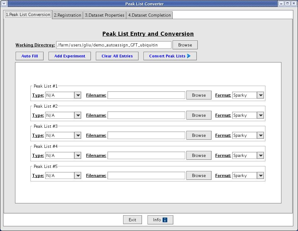
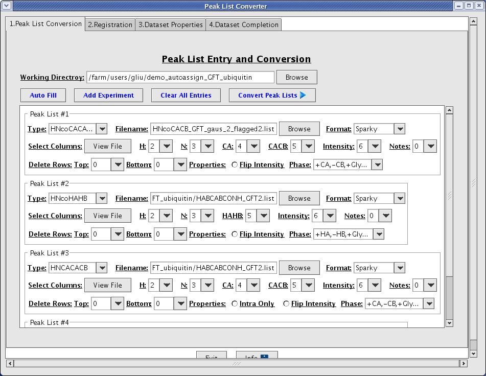
The peak list conversion process is designed to reformat given peak lists into AutoAssign format (Figure 3).  Here the user defines the columns and spectral properties of each peak list.

Figure 3:  Peak List Conversion Page

• Working directory [text field]: it is a base directory that the interface will use to create a subdirectory with a time stamp. The default is set to the current working directory.
• Auto Fill [button]: when a user decides to reuse the same peak lists or the same type of configuration based on the previous analysis, this function allows a user to import the data previously used.
• Add Experiment [button]: This function allows a user to display additional blank peaklist panel.
• Clear All Entries [button]: this function clears populated data fields displayed on screens.
• Convert Peak Lists [button]: this function runs a set of AutoAssign perl scripts to converts peak lists entered by a user. It generates intermediate files used to compute registration/tolerance values for the subsequent steps. All scripts executions run by interface is logged in event.log file found under the subdirectory named with a time stamp along with other intermediate files.
  

Registration

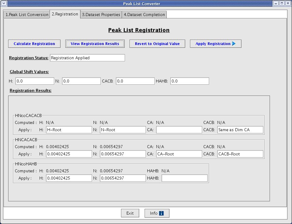
A user will be taken to the Registration tab when Convert Peak List button is clicked. This will allow a user to calculate registration values and apply those values to shift peaks by creating new / temporal peaklist files (Figure 4).

Figure 4: Peak List Registration Page

• Calculate Registration [button]: this function starts calculating registration value and it will open a progress monitor window to notify you how many calculations are completed. The error may be recorded in .reg file(s) under subdirectory if it occurs.
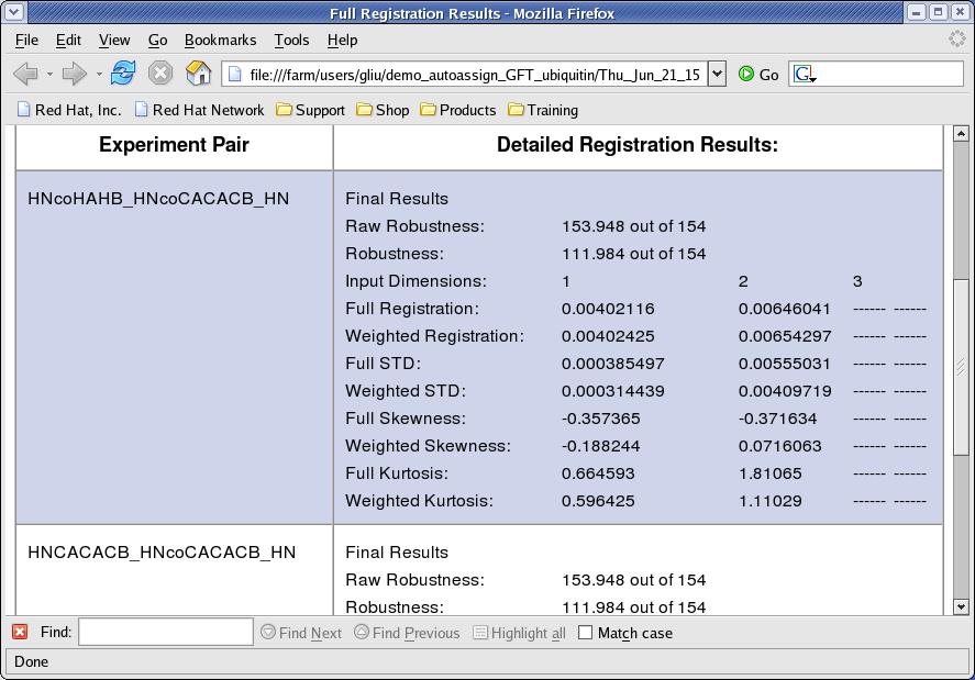
• View Registration [button]: the interface will create an html page by consolidating .reg files generated and will try to open it with a browser. The Weighted Registration values are used to register peak lists. The Full Std values are used in calculating tolerances included in the control file (Figure 5).
  
• Revert to Original Value [button]: this function refills text fields for registration value with original registration value calculated.
• Apply Registration [button]: this function applies registration values to each peaklist. It creates new peaklist files with _shifted.pks extension.

Figure 5: Registration Results Page

Dataset Properties

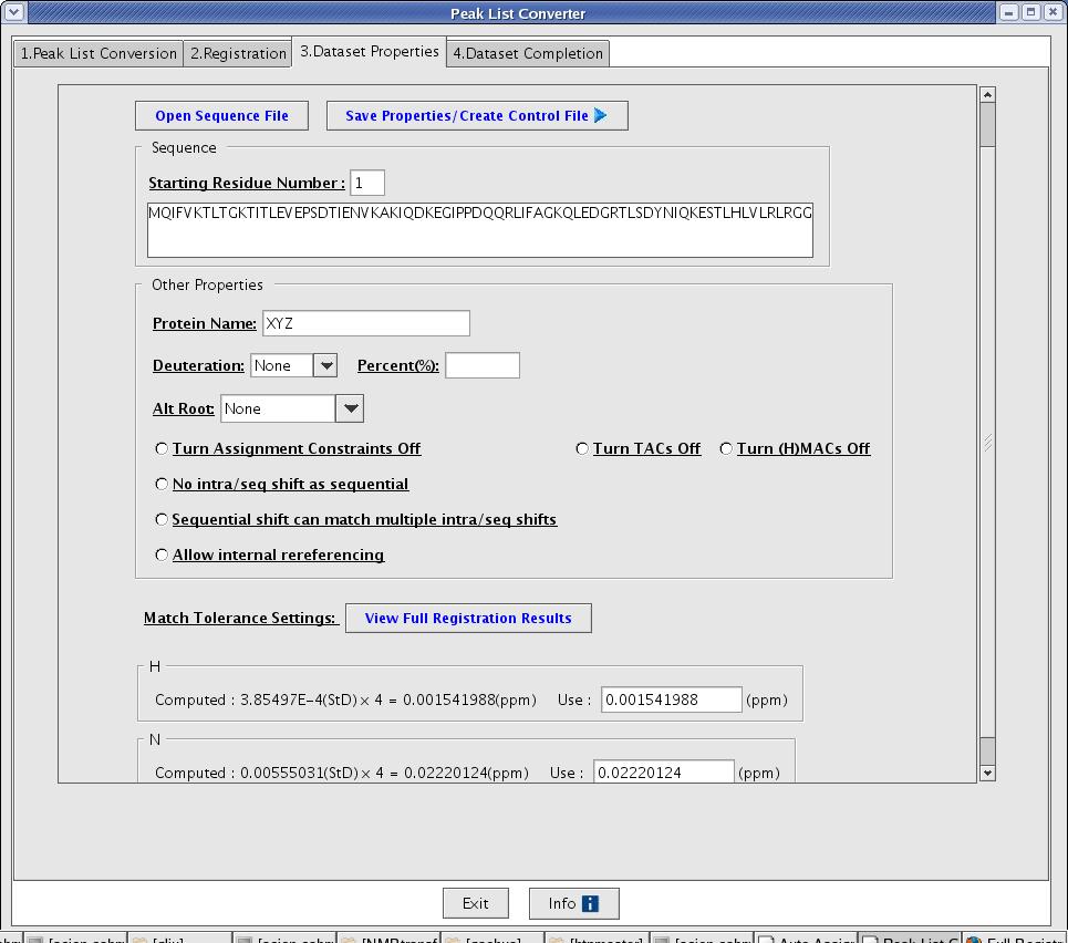
After registration, the converter moves to the Data Set Properties page (Figure 6). A user is asked to provide additional information to complete the control file creation. The value entered by a user on this tab will be used in the properties, tolerances and sequence sections in a control file.

• Open Sequence File [button]: this function opens a window for a user to select a sequence file.
• Save Properties/Create Control File [button]: this function saves dataset property information into an internal data structure and use it to produce a control file. This button should be clicked to produce an initial control file and the result will be displayed on the next tab.

Figure 6:  Data Set Properties Page

Dataset Completion

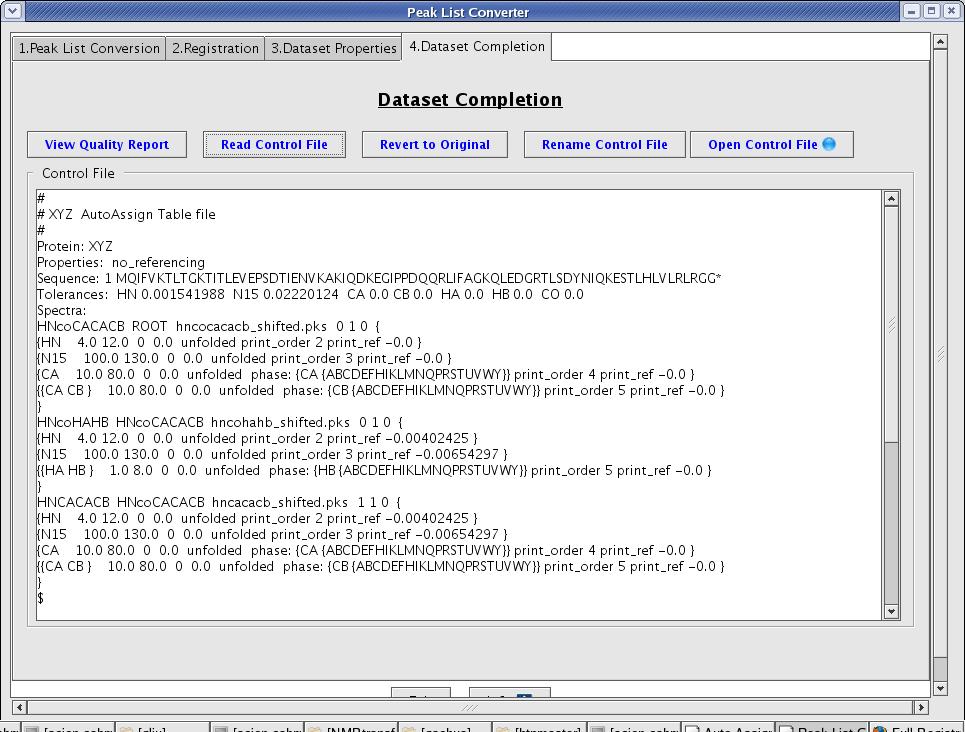
A user can review the control file generated by the interface, manually edit its content, and then save it (Figure 7). To save a revised control file select the Rename Control File button. 

• View Quality Report [button]: this function opens a window for a user to view quality assessment report on the dataset.
• Read Control File [button]: this function allows a user to import an existing control file to view.
• Revert to Original [button]: this function brings back original control file to the screen.
• Rename Control File [button]: this function allows to save a control file with a different name.
• Open Control File [button]: this function opens a control file for analysis. The default control file is the one with original values. When a user saved the control file, that file becomes the default.

Figure 7:  Peak List Converter Page

Follow the Dataset Creation process that the interface guides you through. At the end, you will have a dataset in AutoAssign format.  Hitting the Open Control File button launches a new AutoAssign connectivity map window, and the user can proceed to computing resonance assignments.

Manually Preparation of Peak Files (UB)

One can manually prepare input files by using the follow format, UBNMR can also be used to prepare the input files for AutoAssign. In UBNMR run makeAutoList to generate input files for AutoAssign.

• Peak File Format:
  

  <Index>     <dim1>     <dim2>     [dimX]     <Intensity>     <Label>[.PeakNotes]

...

• Here is an example HNCA peak list file:
  

      #Index   Xppm     Yppm     Zppm     Intensity    Label.notes

   126     8.871      110.859   50.247   3242120        HNCA
   125     8.870      110.898   62.529   724463         HNCA.;g45
   73       8.744      116.161   56.614   2287600       HNCA
   :
   :

145 9.153 112.004 57.415 2788050 HNCA
where individual fields are separated by spaces and/or tabs, and comments are indicated by a "#" sign at the beginning of a line.

Performing Resonance Assignments

Connect to the server and open control-file

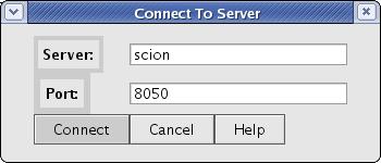
• One can open a dataset to analyze start from the main menu by selecting File+ -> =Open Control File menu option or pressing the Open Control File button on the 4th tab (dataset completion) of the Dataset Creation Graphical User Interface.
• AutoAssign will bring up the following window prompting the user to connect to a server (Figure 8):
  

Figure 8: Connection to Server

If the client and server are on the same computer, you should be able to simply select "Connect".

• Next a blank Connectivity Map window is opened (Figure 9).

Starting a Backbone Resonance Assignment

Select the Execute -> Default Execution menu option to start the analysis.

• Default Execution is the suggested method to run the program. The Refined Execution Execute menu option run AutoAssign in an aggressive mode which is not as safe as the Default Execution option.
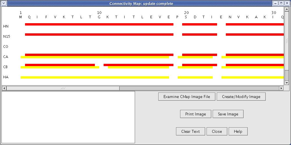
• The Connectivity Map will show the resonance assignment results as the analysis progresses. The whole analysis should only take a few seconds (Figure 10).

Figure 10:  Assigned Connectivity Map

Examining and Saving the Resonance Assignment Results

1. The saving format options can be selected under the save -> Chemical Shift submenus.
2. The Specific GS, Unassigned Residues, and Unassigned GSs Examine menu options are very valuable to troubleshoot problems with assignments or missing assignments. These can be as guides to reexamine spectra to find missing peaks or to apply peak-based assignment constraints if such interventions are necessary.
3. The results file saved from Examine -> All GSs is used to convert the AutoAssign result to XEASY. 
4. For individually assigned peak lists in Sparky format click:  Save -> All Sparky Peaklists.
5. There are several options under Save -> Chemical Shifts for saving the assignments in bmrb formats (2.1 and 3.0) and connectivity map format (cmap).
   

References ==

1.   Zimmerman, D.E., Kulikowski, C.A., Huang, Y., Feng, W., Tashiro, M.,  Shimotakahara, S., Chien, C., Powers, R. and Montelione, G.T. (1997) Automated analysis of protein NMR assignments using methods from artificial intelligence. J. Mol. Biol. 269, 592-610.