Side chain assignment with aliphatic (4,3)D HCCH-COSY in XEASY: Difference between revisions
No edit summary |
No edit summary |
||
| Line 10: | Line 10: | ||
#Go to <tt>analysis/xeasy/hcchcosy</tt>.In UBNMR, run <tt>makeCosyPeak</tt> to generate an extended AtomList as <tt>bbscgftI1.prot</tt> which contains all required linear combinations to assign more peripheral aliphatic spins; A complete starting HC-peak list as <tt>hcchcosyI1.peaks</tt> is generated for analysis of (4,3)D HCCH, taking averaged HG/CG-, HD/CD-, HE/Main.CE- shifts from the BMRB for thus far unassigned side-chain chemical shifts. Peaks predicted based on the BMRB shifts are colored according to being detected on =HG/CG=-,=HD/CD=-,=HE/Main.CE=-moieties. | #Go to <tt>analysis/xeasy/hcchcosy</tt>.In UBNMR, run <tt>makeCosyPeak</tt> to generate an extended AtomList as <tt>bbscgftI1.prot</tt> which contains all required linear combinations to assign more peripheral aliphatic spins; A complete starting HC-peak list as <tt>hcchcosyI1.peaks</tt> is generated for analysis of (4,3)D HCCH, taking averaged HG/CG-, HD/CD-, HE/Main.CE- shifts from the BMRB for thus far unassigned side-chain chemical shifts. Peaks predicted based on the BMRB shifts are colored according to being detected on =HG/CG=-,=HD/CD=-,=HE/Main.CE=-moieties. | ||
#In XEASY, use <tt>ns</tt> to load HCCH sub-spectrum I (comprising peaks at <tt>w2(13C+1H)</tt>), sub-spectrum II (comprising peaks at <tt>w2(13C-1H)</tt>), and the central peak sub-spectrum; use <tt>ls</tt>, <tt>lc</tt> and <tt>lp</tt> to load the corresponding SequenceList <tt>protein.seq</tt> AtomList <tt>bbscgftI1.prot</tt> and starting PeakList <tt>hcchcosyI1.peaks</tt>; use <tt>dw</tt> to set the displayed color for different types of peaks; use <tt>sp</tt> to select the peaks for display. | #In XEASY, use <tt>ns</tt> to load HCCH sub-spectrum I (comprising peaks at <tt>w2(13C+1H)</tt>), sub-spectrum II (comprising peaks at <tt>w2(13C-1H)</tt>), and the central peak sub-spectrum; use <tt>ls</tt>, <tt>lc</tt> and <tt>lp</tt> to load the corresponding SequenceList <tt>protein.seq</tt> AtomList <tt>bbscgftI1.prot</tt> and starting PeakList <tt>hcchcosyI1.peaks</tt>; use <tt>dw</tt> to set the displayed color for different types of peaks; use <tt>sp</tt> to select the peaks for display. | ||
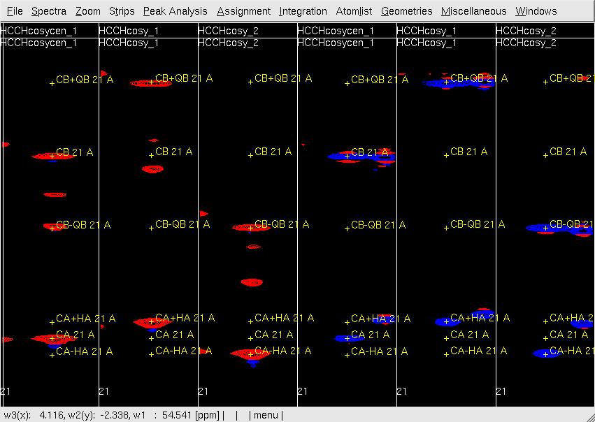
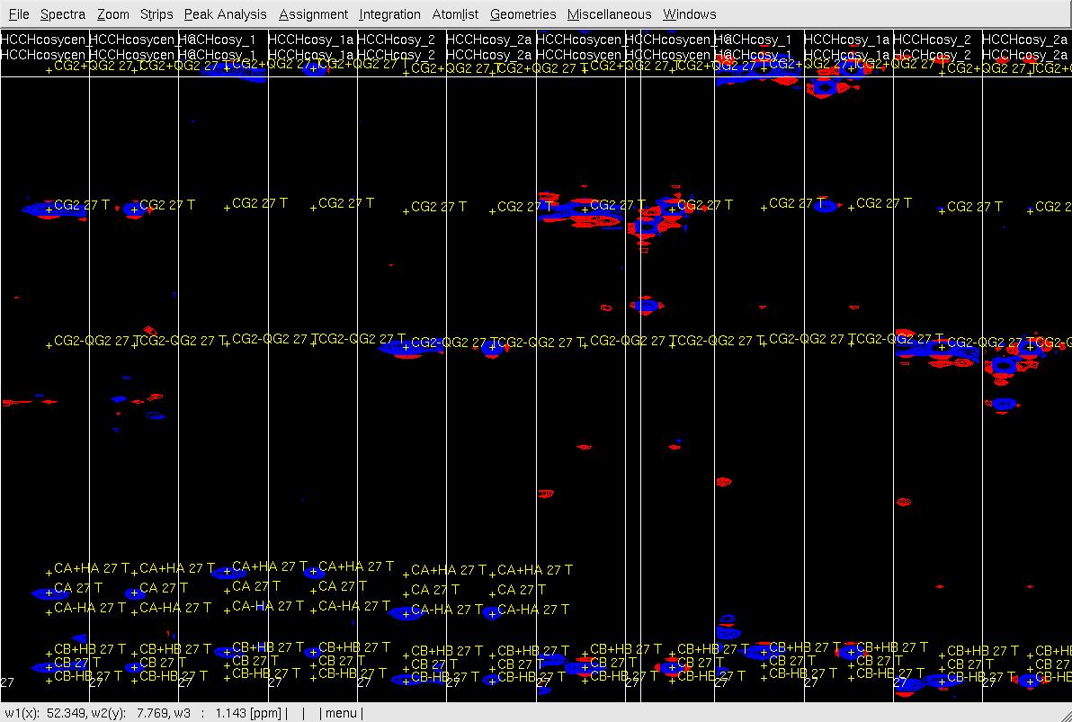
#In XEASY, use <tt>cp</tt> to display the sub-spectra as countour plots; use <tt>es</tt>, <tt>se</tt>, <tt>rs</tt>, <tt>se</tt>, <tt>rs</tt>, <tt>se</tt> and <tt>gs</tt> to create strips for all three spectra (used <tt>rs</tt> here to change the spectra, followed by <tt>se</tt> to search and sort strips) and display strips in the order of residue sequence (Figure 1). <br> '''Figure 1. Example of GFT (4,3)D HCCH analysis.''' Side by side [w2(13C;1H),w3(1HA)]-strip view of (4,3)D HCCH spectra in the order of central spectum and two basic spectra (sub-spectrum I and II). <br> [[ | #In XEASY, use <tt>cp</tt> to display the sub-spectra as countour plots; use <tt>es</tt>, <tt>se</tt>, <tt>rs</tt>, <tt>se</tt>, <tt>rs</tt>, <tt>se</tt> and <tt>gs</tt> to create strips for all three spectra (used <tt>rs</tt> here to change the spectra, followed by <tt>se</tt> to search and sort strips) and display strips in the order of residue sequence (Figure 1). <br> '''Figure 1. Example of GFT (4,3)D HCCH analysis.''' Side by side [w2(13C;1H),w3(1HA)]-strip view of (4,3)D HCCH spectra in the order of central spectum and two basic spectra (sub-spectrum I and II). <br> [[Image:XEASY cos1.jpg]] <br> <br> | ||
#In XEASY, for each residue start with [w2(13C;1H),w3(1HA)]-strip containing signals detected on 1HA (refered to in the following as <tt>HA strip</tt>). Provided that backbone and CB/HB chemical shifts were accurately obtained in previous steps, each HA strip in the basic spectra of (4,3)D HCCH should have peaks accurately positioned at w(13CA +- 1HA) and w(13CB +- 1HB) along w2 (the <tt>GFT dimension</tt>) as shown in Figure 1. In case peaks are not accurately positioned, use <tt>mr</tt> along X-axis (w3(HA)) or Y-axis (w2(13C;1H)) to move peaks to the correct position. After adjusting all peaks of all <tt>HA strips</tt>, use <tt>ac</tt>, <tt>wc</tt> and <tt>wp</tt> to save updated AtomList and Peaklist. If the expected CA shift definig the <tt>13C-plane</tt> of the peaks is different from the actually observed shift along w2(13C), peak positions need to be adjusted the correct plane; use <tt>fp</tt> and <tt>bp</tt> to search for correct plane; use <tt>pm</tt> and <tt>gs</tt> to display [w2(13C;1H),w1(13CA)]-strips (shown in Figure 2); use <tt>mr</tt> to move the peaks along X-axis( w1(13C)) into the correct 13C-shift. If two B-proton shifts are apparently degenerate, move both corresponding peaks to the same position (note that in better resolved NOESY the two shifts may appear to be non-degenerate). <br> '''Figure 2. Example of GFT (4,3)D HCCH analysis.''' Side by side [w2(13C;1H),w1(13C)]-strip view of (4,3)D HCCH spectra in the order of central spectum and two basic spectra (sub-spectrum I and II). <br> [[ | #In XEASY, for each residue start with [w2(13C;1H),w3(1HA)]-strip containing signals detected on 1HA (refered to in the following as <tt>HA strip</tt>). Provided that backbone and CB/HB chemical shifts were accurately obtained in previous steps, each HA strip in the basic spectra of (4,3)D HCCH should have peaks accurately positioned at w(13CA +- 1HA) and w(13CB +- 1HB) along w2 (the <tt>GFT dimension</tt>) as shown in Figure 1. In case peaks are not accurately positioned, use <tt>mr</tt> along X-axis (w3(HA)) or Y-axis (w2(13C;1H)) to move peaks to the correct position. After adjusting all peaks of all <tt>HA strips</tt>, use <tt>ac</tt>, <tt>wc</tt> and <tt>wp</tt> to save updated AtomList and Peaklist. If the expected CA shift definig the <tt>13C-plane</tt> of the peaks is different from the actually observed shift along w2(13C), peak positions need to be adjusted the correct plane; use <tt>fp</tt> and <tt>bp</tt> to search for correct plane; use <tt>pm</tt> and <tt>gs</tt> to display [w2(13C;1H),w1(13CA)]-strips (shown in Figure 2); use <tt>mr</tt> to move the peaks along X-axis( w1(13C)) into the correct 13C-shift. If two B-proton shifts are apparently degenerate, move both corresponding peaks to the same position (note that in better resolved NOESY the two shifts may appear to be non-degenerate). <br> '''Figure 2. Example of GFT (4,3)D HCCH analysis.''' Side by side [w2(13C;1H),w1(13C)]-strip view of (4,3)D HCCH spectra in the order of central spectum and two basic spectra (sub-spectrum I and II). <br> [[Image:XEASY cos2.jpg]]<br> <br> | ||
#In UBNMR, run <tt>updatecosyGFT</tt> to update the SQ chemical shifts as <tt>hcchcosyI2.prot</tt> and re-generate a new peak list <tt>hcchcosyI2.peaks</tt> to proceed further with side-chain assignments. | #In UBNMR, run <tt>updatecosyGFT</tt> to update the SQ chemical shifts as <tt>hcchcosyI2.prot</tt> and re-generate a new peak list <tt>hcchcosyI2.peaks</tt> to proceed further with side-chain assignments. | ||
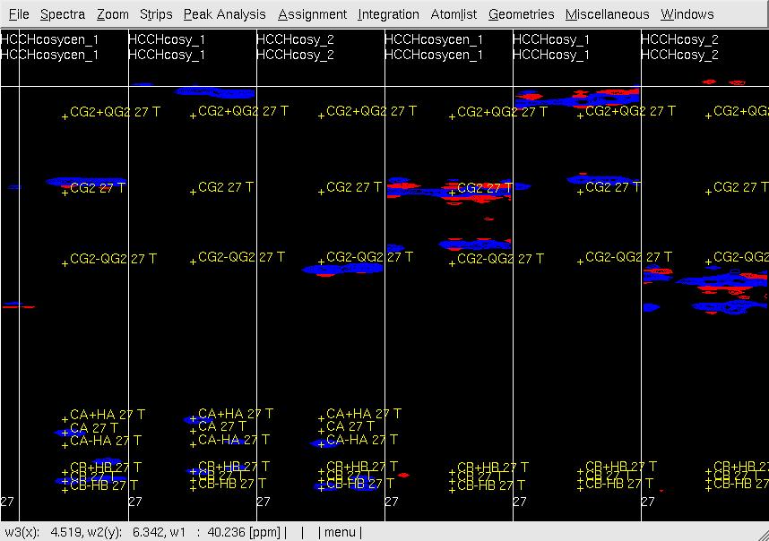
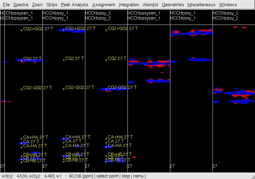
#In XEASY, use <tt>lp</tt> to re-load the PeakList; <tt>es</tt>, <tt>se</tt>; and <tt>gs</tt>; to re-sort the strips of the three sub-spectra as described above; use <tt>sf</tt> to display the [w1(13C;1H),w3(1HB)]-strip (<tt>CB/HB strips</tt>). The peaks are colored according to the proton on which signals are detected, that is, different colors are used for peaks detected on A-, B-, G-, D-, and E- protons; use <tt>mr</tt> to accurately position peaks at w(13CG) and w(13CG+-1HG) (Figure 3); use <tt>ac</tt>, <tt>wc</tt> and <tt>wp</tt> to save updated AtomList <tt>hcchcosyO2.prot</tt> and PeakList <tt>hcchcosyO2.peaks</tt>. <br> '''Figure 3 Example of GFT (4,3)D HCCH analysis.''' Side by side [w2(13C;1HB),w3(1HB)]-strip view of (4,3)D HCCH spectra in the order of central spectum and two basic spectra (sub-spectrum I and II) before (left) and after (right) peak position adjustment of w(13CG) and w(13CG+-1HG). <br> [[ | #In XEASY, use <tt>lp</tt> to re-load the PeakList; <tt>es</tt>, <tt>se</tt>; and <tt>gs</tt>; to re-sort the strips of the three sub-spectra as described above; use <tt>sf</tt> to display the [w1(13C;1H),w3(1HB)]-strip (<tt>CB/HB strips</tt>). The peaks are colored according to the proton on which signals are detected, that is, different colors are used for peaks detected on A-, B-, G-, D-, and E- protons; use <tt>mr</tt> to accurately position peaks at w(13CG) and w(13CG+-1HG) (Figure 3); use <tt>ac</tt>, <tt>wc</tt> and <tt>wp</tt> to save updated AtomList <tt>hcchcosyO2.prot</tt> and PeakList <tt>hcchcosyO2.peaks</tt>. <br> '''Figure 3 Example of GFT (4,3)D HCCH analysis.''' Side by side [w2(13C;1HB),w3(1HB)]-strip view of (4,3)D HCCH spectra in the order of central spectum and two basic spectra (sub-spectrum I and II) before (left) and after (right) peak position adjustment of w(13CG) and w(13CG+-1HG). <br> [[Image:XEASY cos4.jpg]] [[Image:XEASY cos3.jpg]] <br> <br> | ||
#In UBNMR, run <tt>updatecosyGFT</tt> to update the SQ shifts and to generate a PeakList (e.g. <tt>hcchcosyI3.peaks</tt>) using updated shifts. | #In UBNMR, run <tt>updatecosyGFT</tt> to update the SQ shifts and to generate a PeakList (e.g. <tt>hcchcosyI3.peaks</tt>) using updated shifts. | ||
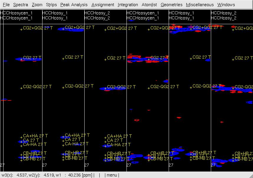
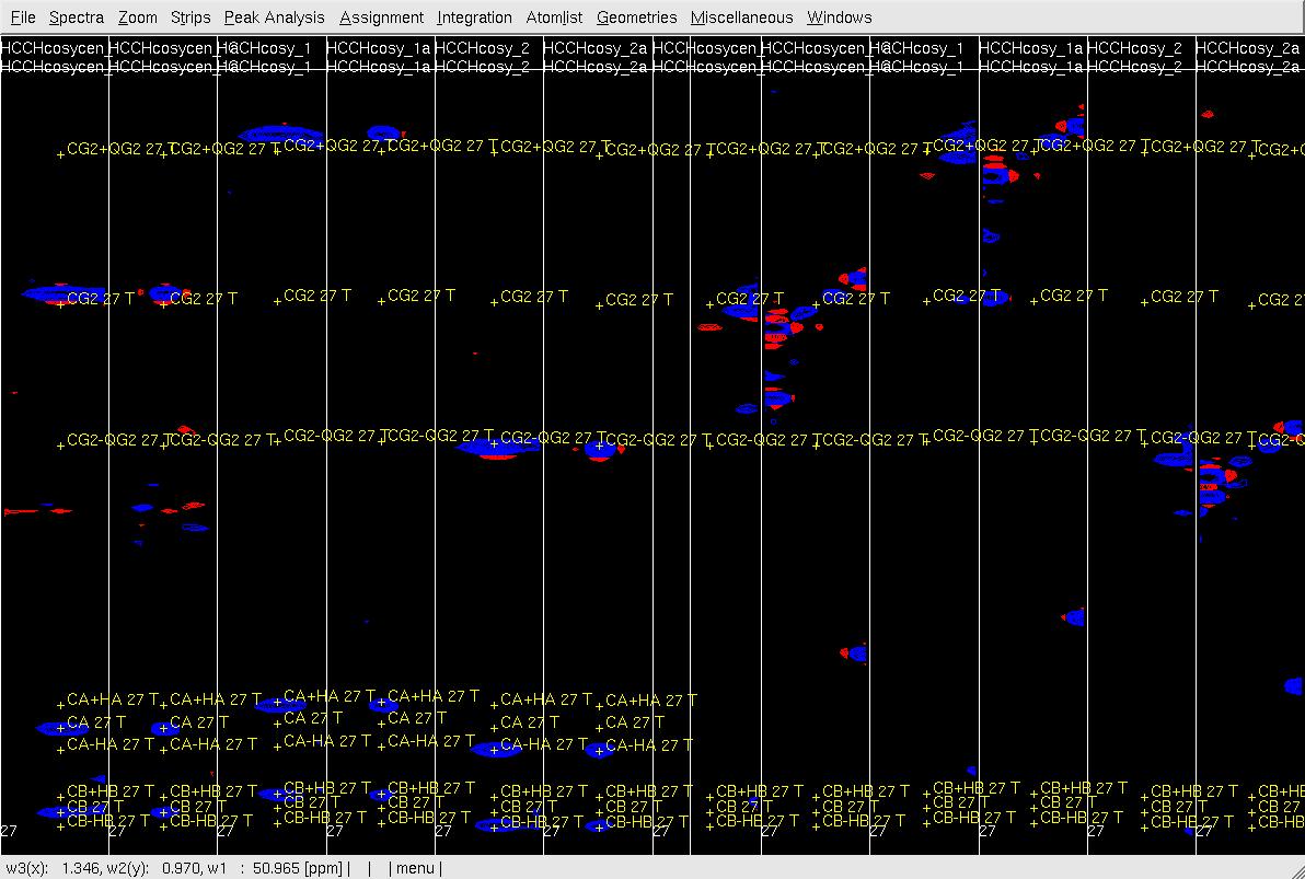
#In XEASY, repeat step 6 for [w1(13C;1H),w3(1HG)]-strips (<tt>CG/HG strips</tt>) to confirm peaks accurately positioned at w(13CG+- 1HG) as show in Figure 4, re-adjust the peak position if necessary. <br> '''Figure 4 Example of GFT (4,3)D HCCH analysis.''' Side by side [w2(13C;1HB),w3(1HB)] (first three strips) and [w2(13C;1HG),w3(1HG)] (later three stips) strips view of (4,3)D HCCH spectra in the order of central spectum and two basic spectra (sub-spectrum I and II). '''Top:''' before peak position adjustment and before updating shifts of w(13CG) and w(13CG+-1HG); '''Middle:''' after peak position adjustment and before updating shifts of w(13CG) and w(13CG+-1HG); '''Bottom:''' after peak position adjustment and after updating shifts of w(13CG) and w(13CG+-1HG). <br> <br> [[ | #In XEASY, repeat step 6 for [w1(13C;1H),w3(1HG)]-strips (<tt>CG/HG strips</tt>) to confirm peaks accurately positioned at w(13CG+- 1HG) as show in Figure 4, re-adjust the peak position if necessary. <br> '''Figure 4 Example of GFT (4,3)D HCCH analysis.''' Side by side [w2(13C;1HB),w3(1HB)] (first three strips) and [w2(13C;1HG),w3(1HG)] (later three stips) strips view of (4,3)D HCCH spectra in the order of central spectum and two basic spectra (sub-spectrum I and II). '''Top:''' before peak position adjustment and before updating shifts of w(13CG) and w(13CG+-1HG); '''Middle:''' after peak position adjustment and before updating shifts of w(13CG) and w(13CG+-1HG); '''Bottom:''' after peak position adjustment and after updating shifts of w(13CG) and w(13CG+-1HG). <br> <br> [[Image:XEASY cos5.jpg]]<br> <br> [[Image:XEASY cos6.jpg]] <br> <br> [[Image:XEASY cos7.jpg]] <br> <br> <br> | ||
#In UBNMR, run <tt>updatecosyGFT</tt> to update SQ shifts and to generate a PeakList (e.g. <tt>hcchcosyI4.peaks</tt>) using updated shifts. | #In UBNMR, run <tt>updatecosyGFT</tt> to update SQ shifts and to generate a PeakList (e.g. <tt>hcchcosyI4.peaks</tt>) using updated shifts. | ||
#In XEASY, for peripheral nuclei beyond CD, repeat steps 6-8 for [w1(13C;1H),w3(1HD)]-strips (<tt>CD/HD strips</tt>) to obtain peaks accurately positioned at w(13CD+- 1HD). | #In XEASY, for peripheral nuclei beyond CD, repeat steps 6-8 for [w1(13C;1H),w3(1HD)]-strips (<tt>CD/HD strips</tt>) to obtain peaks accurately positioned at w(13CD+- 1HD). | ||
| Line 23: | Line 23: | ||
#In UBNMR, run <tt>cleanCosyGft</tt>. The AtomList is loaded, SQ 1H and 13C are calculated and written into the AtomList while all linear combinations of shifts are removed. The thus generated final SQ-only AtomList as <tt>bbsc.prot</tt> contains all shifts and represents the starting point for analysis of NOESY. <br> <br> | #In UBNMR, run <tt>cleanCosyGft</tt>. The AtomList is loaded, SQ 1H and 13C are calculated and written into the AtomList while all linear combinations of shifts are removed. The thus generated final SQ-only AtomList as <tt>bbsc.prot</tt> contains all shifts and represents the starting point for analysis of NOESY. <br> <br> | ||
<br> | <br> | ||
=== '''Approach II, using <tt>mr</tt> to find the SQ chemical shift''' === | === '''Approach II, using <tt>mr</tt> to find the SQ chemical shift''' === | ||
Latest revision as of 22:50, 11 November 2009
Aliphatic Side-chain Resonance Assignment Using the Aliphatic HCCHCOSY Spectrum
The sequence specific 15N /1HN /13CAB resonance assignments obtained as described in Backbone Assignment are first used to also obtain 1HA and 1HB Assignment by analyzing (4,3)D HABCAB(CO)NHN. Then, shifts of more peripheral aliphatic spins are obtained from (4,3)D HCCH or other spectra. Two approaches by using (4,3)D HCCH are described below and the later one requires more experience. NOTE: Here atom A, B, G, D, E stand for atom alpha α, beta β, gama γ, delta δ, and epsilon ε. Dimensions of HCCH are w1, 13C; _w2, (13C+-1H), the GFT dimension;_ and w3, 1H, direct detect dimension.
Approach I, using UBNMR to update SQ chemical shift
- Go to analysis/xeasy/hcchcosy.In UBNMR, run makeCosyPeak to generate an extended AtomList as bbscgftI1.prot which contains all required linear combinations to assign more peripheral aliphatic spins; A complete starting HC-peak list as hcchcosyI1.peaks is generated for analysis of (4,3)D HCCH, taking averaged HG/CG-, HD/CD-, HE/Main.CE- shifts from the BMRB for thus far unassigned side-chain chemical shifts. Peaks predicted based on the BMRB shifts are colored according to being detected on =HG/CG=-,=HD/CD=-,=HE/Main.CE=-moieties.
- In XEASY, use ns to load HCCH sub-spectrum I (comprising peaks at w2(13C+1H)), sub-spectrum II (comprising peaks at w2(13C-1H)), and the central peak sub-spectrum; use ls, lc and lp to load the corresponding SequenceList protein.seq AtomList bbscgftI1.prot and starting PeakList hcchcosyI1.peaks; use dw to set the displayed color for different types of peaks; use sp to select the peaks for display.
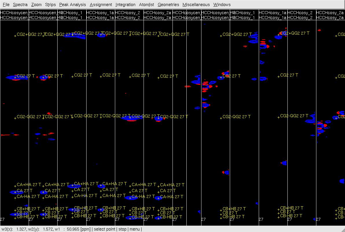
- In XEASY, use cp to display the sub-spectra as countour plots; use es, se, rs, se, rs, se and gs to create strips for all three spectra (used rs here to change the spectra, followed by se to search and sort strips) and display strips in the order of residue sequence (Figure 1).
Figure 1. Example of GFT (4,3)D HCCH analysis. Side by side [w2(13C;1H),w3(1HA)]-strip view of (4,3)D HCCH spectra in the order of central spectum and two basic spectra (sub-spectrum I and II).
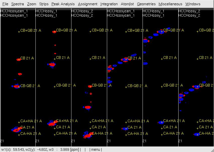
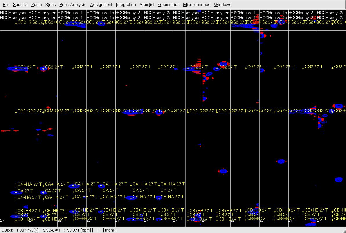
- In XEASY, for each residue start with [w2(13C;1H),w3(1HA)]-strip containing signals detected on 1HA (refered to in the following as HA strip). Provided that backbone and CB/HB chemical shifts were accurately obtained in previous steps, each HA strip in the basic spectra of (4,3)D HCCH should have peaks accurately positioned at w(13CA +- 1HA) and w(13CB +- 1HB) along w2 (the GFT dimension) as shown in Figure 1. In case peaks are not accurately positioned, use mr along X-axis (w3(HA)) or Y-axis (w2(13C;1H)) to move peaks to the correct position. After adjusting all peaks of all HA strips, use ac, wc and wp to save updated AtomList and Peaklist. If the expected CA shift definig the 13C-plane of the peaks is different from the actually observed shift along w2(13C), peak positions need to be adjusted the correct plane; use fp and bp to search for correct plane; use pm and gs to display [w2(13C;1H),w1(13CA)]-strips (shown in Figure 2); use mr to move the peaks along X-axis( w1(13C)) into the correct 13C-shift. If two B-proton shifts are apparently degenerate, move both corresponding peaks to the same position (note that in better resolved NOESY the two shifts may appear to be non-degenerate).
Figure 2. Example of GFT (4,3)D HCCH analysis. Side by side [w2(13C;1H),w1(13C)]-strip view of (4,3)D HCCH spectra in the order of central spectum and two basic spectra (sub-spectrum I and II).
- In UBNMR, run updatecosyGFT to update the SQ chemical shifts as hcchcosyI2.prot and re-generate a new peak list hcchcosyI2.peaks to proceed further with side-chain assignments.
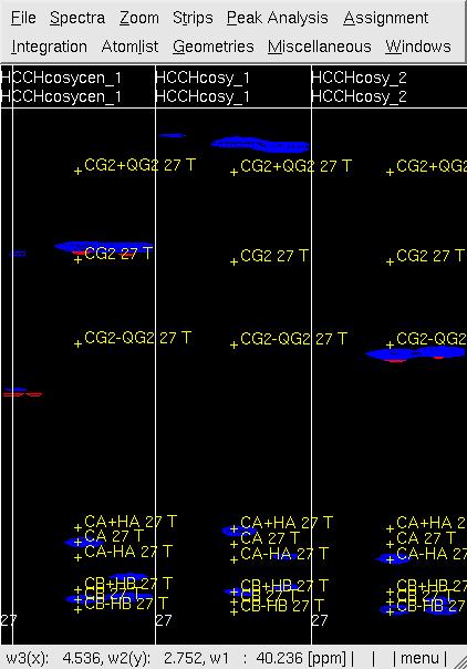
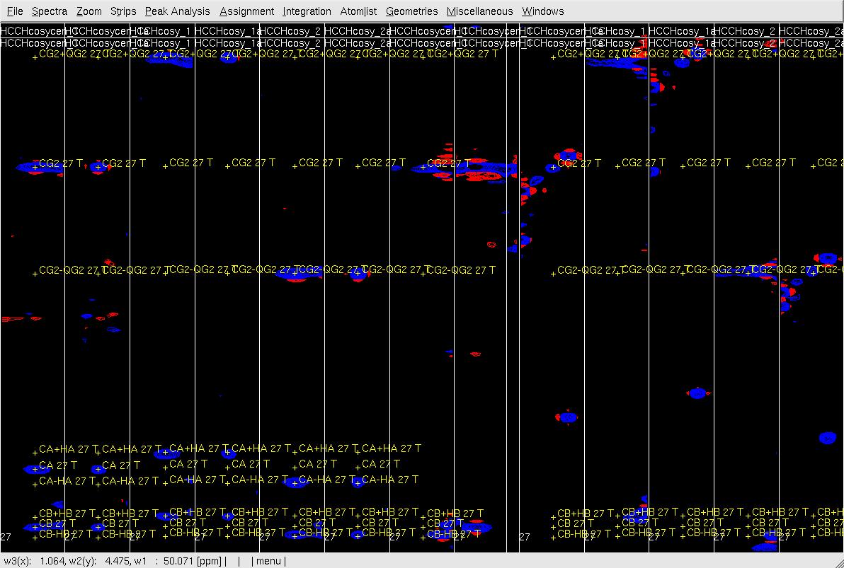
- In XEASY, use lp to re-load the PeakList; es, se; and gs; to re-sort the strips of the three sub-spectra as described above; use sf to display the [w1(13C;1H),w3(1HB)]-strip (CB/HB strips). The peaks are colored according to the proton on which signals are detected, that is, different colors are used for peaks detected on A-, B-, G-, D-, and E- protons; use mr to accurately position peaks at w(13CG) and w(13CG+-1HG) (Figure 3); use ac, wc and wp to save updated AtomList hcchcosyO2.prot and PeakList hcchcosyO2.peaks.
Figure 3 Example of GFT (4,3)D HCCH analysis. Side by side [w2(13C;1HB),w3(1HB)]-strip view of (4,3)D HCCH spectra in the order of central spectum and two basic spectra (sub-spectrum I and II) before (left) and after (right) peak position adjustment of w(13CG) and w(13CG+-1HG).
- In UBNMR, run updatecosyGFT to update the SQ shifts and to generate a PeakList (e.g. hcchcosyI3.peaks) using updated shifts.
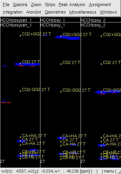
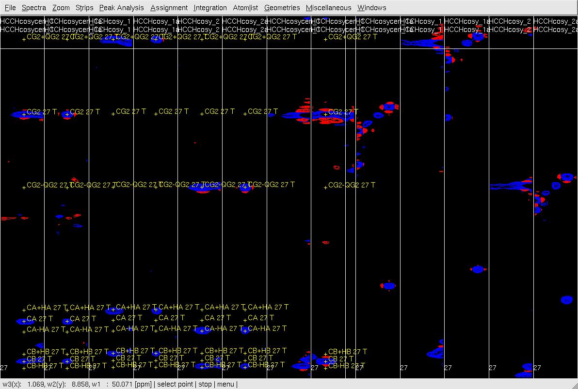
- In XEASY, repeat step 6 for [w1(13C;1H),w3(1HG)]-strips (CG/HG strips) to confirm peaks accurately positioned at w(13CG+- 1HG) as show in Figure 4, re-adjust the peak position if necessary.
Figure 4 Example of GFT (4,3)D HCCH analysis. Side by side [w2(13C;1HB),w3(1HB)] (first three strips) and [w2(13C;1HG),w3(1HG)] (later three stips) strips view of (4,3)D HCCH spectra in the order of central spectum and two basic spectra (sub-spectrum I and II). Top: before peak position adjustment and before updating shifts of w(13CG) and w(13CG+-1HG); Middle: after peak position adjustment and before updating shifts of w(13CG) and w(13CG+-1HG); Bottom: after peak position adjustment and after updating shifts of w(13CG) and w(13CG+-1HG).
- In UBNMR, run updatecosyGFT to update SQ shifts and to generate a PeakList (e.g. hcchcosyI4.peaks) using updated shifts.
- In XEASY, for peripheral nuclei beyond CD, repeat steps 6-8 for [w1(13C;1H),w3(1HD)]-strips (CD/HD strips) to obtain peaks accurately positioned at w(13CD+- 1HD).
- In UBNMR, run updatecosyGFT to update SQ shifts and to generate a PeakList (e.g. hcchcosyI5.peaks) using updated shifts.
- In XEASY, for Main.CE, repeat steps 6-8, confirm that peaks are accurately positioned in [w1(13C;1H),w3(1HE)]-strips (Main.CE/HE strips) at w(13Main.CE+-E 1HE).
- In XEASY, use ac, wc and wp to save final AtomList (e.g. hcchcosyO5.prot) and PeakList (e.g. hcchcosyO5.peaks).
- In UBNMR, run cleanCosyGft. The AtomList is loaded, SQ 1H and 13C are calculated and written into the AtomList while all linear combinations of shifts are removed. The thus generated final SQ-only AtomList as bbsc.prot contains all shifts and represents the starting point for analysis of NOESY.


Approach II, using mr to find the SQ chemical shift
The procotol describe above updates SQ shifts step by step by using UBNMR, there is another approach that update SQ shifts step by step by directly adjust peak position with two orthognal display of the spectra. The later approach is given below and may require addtional experience.
- In XEASY, use ns to load two copies of the three sub-spectra of (4,3) HCCHand display the two copies in two orthogonal view (X-axis: w3(1H), Y-axis: w2(13C;1H), Z-axis: w1(13C) & X-axis: w3(13C), Y-axis:w2(1H), z: w3(1H)); use ls, lc, and lp, respectively, to load corresponding SequenceList, AtomList and PeakList; use sp, se and gs to display [w3(1H),w2(13C;1H)]-strips and [w1(13C),w2(13C;1H)]-strips for the interested residue.
- In XEASY, start from both views (X-axis: w3(1H), Y-axis: w2(13C;1H), Z-axis: w1(13C) & X-axis: w1(13C), Y-axis, w2(13C;1H), Z-axis: w3(1H)) of both HA and HB strips, confirm the assignment for CA/HA and CB/HB, and re-adjust the peak position if necessarys by using mr. Adjusting peak position along X-axis in strips with view (X-axis: w3(1H), Y-axis: w2(13C;1H), Z-axis: w1(13C) for 1H chemical shift, along X-axis in strips with view (X-axis: w1(13C), Y-axis: w2(13C;1H), Z-axis: w3(1H))for 13C chemical shifts, along Y-axis for GFT chemical shift w(C13;1H).
- In XEASY, go to the CB/HB strips, use mr to accurately position peaks at w(13CG) and w(13CG+-1HG) along Y-axis (Figure 5). While adjusting the peak position, pay attention to wether the chemical shift difference value of (w(13CG+HG) - w(13CG-HG)) become larger or small. In the case of water frenquency as the GFT dimension 1H carrier, the real HG shift is smaller than initial value if the difference become small (more negative).
Figure 5. Example of GFT (4,3)D HCCH analysis. Side by side orthogonal views of [w2(13C;1HB),w3(1HB)] and [w2(13C;1HG),w3(1HG)] strips view of (4,3)D HCCH spectra in the order of X-axis as HB central, CB central, HB sub-spectrum I, CB sub-spectrum I, HB sub-spectrum II, CB sub-spectrum II, HG central, CG central, HG sub-spectrum I, CG sub-spectrum I, HG sub-spectrum II and CG sub-spectrum II. Top: before peak position adjustment of w(13CG) and w(13CG+-1HG); Middle: after peak position adjustment of w(13CG) and w(13CG+-1HG) and before resorting strips; Bottom: after peak position adjustment of w(13CG), and w(13CG+-1HG) and after resorting strips.
- In XEASY use es, se and gs to resort and redisplay the strips in both view. As shown in Figure 6 Top, since the chemical shift of CG is correct, identify the correct HG chemical shift in the HG strip with view (X-axis: w3(13C), Y-axis:w2(1H); z: w3(1H)) based on the expected peak pattern and expected HG peak position. Use zd to duplicate the HG central strip if the expect position of HG is out of this strip view (Figure 6, middle), use gl or gr to change the dulpilicate strip view to find the expected HG.
Figure 6. Example of GFT (4,3)D HCCH analysis. Side by side orthogonal views of [w2(13C;1HB),w3(1HB)] and [w2(13C;1HG),w3(1HG)] strips view of (4,3)D HCCH spectra in the order of X-axis as HB central, CB central, HB sub-spectrum I, CB sub-spectrum I, HB sub-spectrum II, CB sub-spectrum II, HG central (has two HG central in the top and middle figures), CG central, HG sub-spectrum I, CG sub-spectrum I, HG sub-spectrum II and CG sub-spectrum II. Top: after zd, and before peak position adjustment of w(1HG); Middle: after zd, after peak position adjustment of w(1HG) and before resorting strips; Bottom: after peak position adjustment of w(1HG) and after resorting strips.
- In XEASY use es, se and gs to resort and redisplay the strips in both view, and confirm the CG/HG shift if both view.
- In XEASY, repeat the above steps for assignments of peripheral nuclei beyond CG of this residue, such as CD/HD and Main.CE/HE.
- In XEASU, use sp to select peaks for the next residues and repeat the above steps for assignments.
- In XEASY, use ac, wc and wp to save final AtomList and PeakList.
- In UBNMR, run cleanCosyGft. The AtomList is loaded, SQ 1H and 13C are calculated and written into the AtomList while all linear combinations of shifts are removed. The thus generated final SQ-only AtomList as bbsc.prot contains all shifts and represents the starting point for analysis of NOESY.


-- Main.GaohuaLiu - 31 Jan 2007@