RDCvis & KiNG
This page is under construction as of November 1st, 2011.
Draft Outline
Intro to RDCvis
Visualizing the RDC curves in their structural context, especially when combined with other structure quality visualizations allows users to easily identify and study areas of their models which need improvement.
Software for generating RDC visualizations, dubbed RDCvis and built into KiNG (Chen, 2009), requires a PDB format coordinate file and an NMR restraints file (in CNS format) with RDC data. RDCvis outputs the RDC visualizations in kinemage format (Richardson, 1992), as a standalone file that is routinely appended onto an existing multi-model kinemage for viewing in KiNG. These curves plotted using the kinemage graphics format, take advantage of the powerful and extensive infrastructure that already exists for manipulating and viewing kinemages in Mage, KiNG, and KinImmerse (Richardson, 1992; Chen, 2009; Block, 2009).
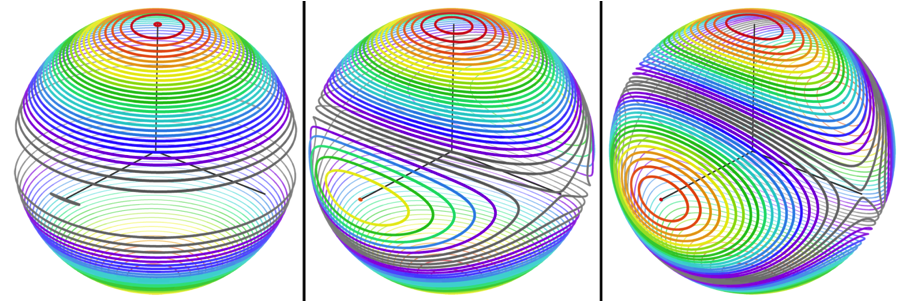
RDCvis draws RDC curves by using singular value decomposition (SVD) (Losonczi, 1999) to calculate a Saupe alignment matrix (Saupe, 1968) from the RDCs. These curves exist on a sphere of all the solutions to the RDC equation (as shown below)
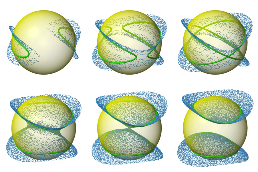
These varied curve shapes - RDC target curves - arise from the intersection of the surface representing the possible solutions for the RDC equation (as shown above) with the sphere representing the possible positions for a given internuclear bond vector, as shown below.
Getting RDCvis to work in KiNG
Walk-through of loading RDCs
Presented here is a walkthrough in KiNG of visualizing RDC’s on an NMR structure ensemble. The example shown is the dvCcmE’ structure determined by the NorthEast Structural Genomics consortium.
What you need
MolProbity multimodel-multicrit kinemage
Multiple models visualized at once with the local geometric and steric validation criteria from the Richardson lab displayed at each residue.
.tbl file (note on acceptible formats
One note is that a significant barrier to using RDCvis is the lack of consistency in the deposited NMR restraints files. A more strictly defined standard data-file format would make RDCvis more straightforward to use and thus routinely useful to a wider community.
PDB file
The PDB file is needed so that RDCvis can calculate the RDCs based off of the coordinates and appropriately drawn them to the kinemage file.
Loading the files - screenshots
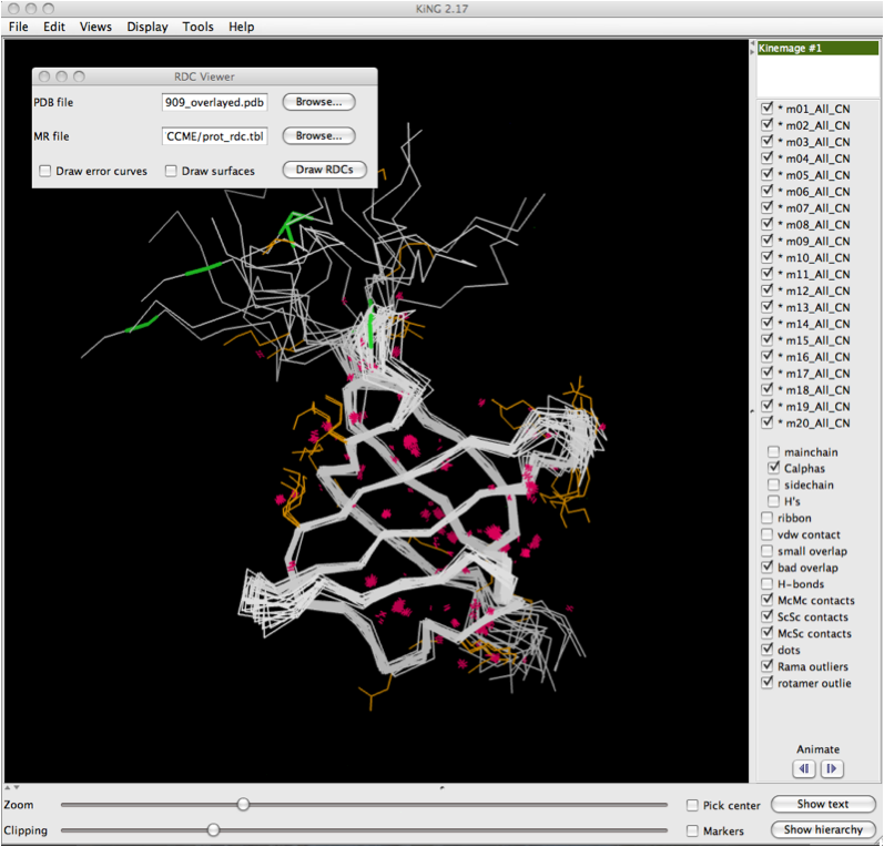
The image below shows the KiNG display software with a multi-model multicrtierion kinemage displayed. The dialog box for RDCvis is present, and there are two files you need to load.: 1) The PDB file (all models) that corresponds to the kinemage you are using. 2) The .tbl file with your RDC data in it.
There are options to draw error curves and to draw all the dot surfaces. Note that dot surfaces can add to compute time and may make the visual field more cluttered. It is, however, useful for making figures of an individual area.
Once the files are properly selected, simply click on 'Draw RDCs'
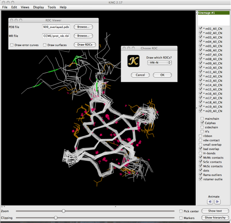
Once you have clicked on the 'Draw RDCs' button, a second dialog box will appear with a drop down menu. This allows you to select which RDCs to draw from the data file. This is particularly useful for structures where mutliple RDCs are present. Note that in order to load multiple RDCs, you must go through this sequence multiple times, once for each set of RDCs you wish to draw. Click 'Ok' once you've selected the RDCs of interest.
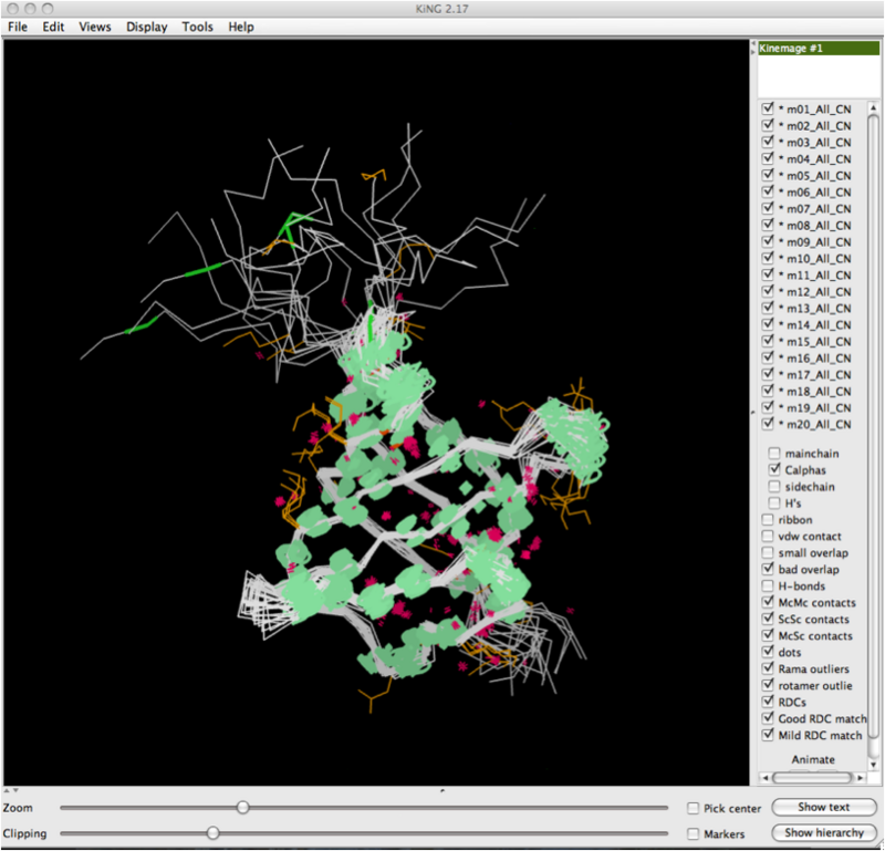
After you've clicked 'Ok', the software will draw the RDCs onto the whole structure. Below shows a zoomed out view of this, and you can observe the RDC curves drawn for every model, at every location where they were observed and the data collected.
Co-centering tool
Translational overlap while maintaining orientation in order to investigate the match of the internuclear vector across all models in the ensemble to the target curves of the measured RDC
In general, even the most well defined NMR ensembles will have enough deviation from model to model that a close-up comparison of the behavior of residues is difficult with an overall superposition. When all models are visible, the visual clutter from all of the models is too overwhelming for reasonable analysis. Viewing models one at a time resolves the issue of clutter, but it is still difficult to compare one model to the others. On-demand local superimposition of the models is one possible solution. However, for visualizing RDC data, which is directly related to the global orientation of the model, any rotation of the models would alter the relationship of the model to the RDCs. Therefore, the co-centering tool translates all the models onto a single point with no rotational aspect in order to maintain the global orientation of the models.
In the majority of cases, co-centering reduces the visual clutter dramatically, allowing for a meaningful observation about the model-by-model agreement of the internuclear bond vector to the RDC curves and a visual assessment the match of the model to the data in the local context. There are some situations where the co-centering may not be enough help. Particularly, in regions where there is a limited amount of experimentally observed data, the different models of the ensemble may have wildly different conformations, which makes co-centering less effective.
Walk through of co-centering tool - screenshots
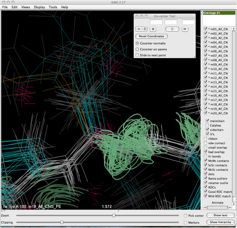
The Co-center tool is found in the Tools -> Kin Editing menu. Clicking on it will bring up the dialog box shown below. In order to co-center, it is helpful to zoom in on the residue or atom of interest and center it in your screen (this eases the selection process and helps reduce visual clutter).
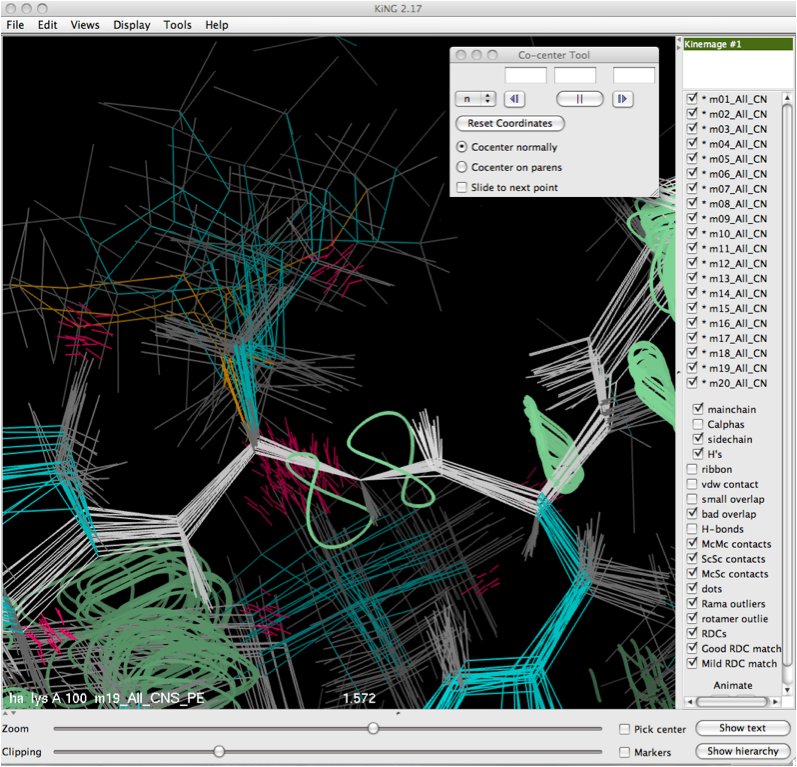
Once the selection is made either by putting it into the dialog box directly, or clicking on it with the mouse, the translational move will be performed and the resulting co-center operation will be performed, leaving the user with a view like that shown below.
Using RDCvis to analyze RDCs in their local context
Analysis with one or multiple RDCs
Just like others have predicted, it is better with multiple RDCs
Even if the tensors are very similar, it can still give useful data to have two RDCs
Philosophically similar to crystallography in that it is looking at validation crteria mapped on a model while also looking at the experimental data (in this case RDCs, in xray it is the density)
Patterns to look for
Orientation Dependent Variability
Contribution from both the orientation of the local structure to the RDC visualized and the RDC visualized to the field.
Implications for flexibility of the internuclear vector
There exists some variation in the internuclear vector match to the RDC data drawn as a curve. This flexibility can result in a fanning out of the internuclear vector along a target curve. The likely contributors to this variation are the “orientation dependent variability,” and the error model of observed RDC’s. I will later discuss modeling the error of the observed RDCs.
Generally, the orientation of the alignment tensor to the molecule (and its rhombicity) will determine the shape of the Saupe curves at each internuclear bond vector where they are experimentally observed. In addition, the orientation of the local structural features of the molecule in relation to the given Saupe curve shape will determine the amount and direction of variation allowable for structural interpretation.
Both orientation of the tensor to the molecule and orientation of the local structural features in relation to the curve interact with one another to impact the potential structural interpretations. For example, if a curve is relatively flat, a peptide rotation approximately around the C direction could swing the NH bond vector along the curve if the curve tangent has the right relationship to the C.
An orientation dependent variability should not be taken to imply dynamics. Rather, it demonstrates that for a given RDC in a local area, there is an arc along which multiple positions remain consistent with the data because of the orientation and shape of the RDC curve in the local environment of the structure model.
One Curve Rule
It can never be on both...
Searching for these systematic errors
Special case where target curves overlap
The usual methodology for use of RDCs in structure solution implicitly assumes one conformation, so that in general a given bond vector should only line up with one or the other curve. Motion or multiple conformations are of course possible, and for loops even probable, but this is not the way to identify such motion. It would require an extremely unlikely coincidence for a motion or conformational change to line up each of two orientational clusters for a given internuclear vector exactly on a different one of the two curves. Even if a residue were sampling conformations that could match both curves, this would result in averaging of the RDC and end up with a different, smaller RDC value. This averaging affect has been treated in the literature, where others have tried to develop a model of conformational sampling that stays in agreement with the observed RDC’s (Clore, 2004; Brooks, 1997; Hess, 2003). We conclude that this behavior in a structure ensemble - of two distinctly different conformations pointing the internuclear vector towards opposite curves - is a potential systematic error allowed by the usual procedure of requiring each individual model to match the scaler RDC value, without considering the relationship of the models to one another or to the target curves.
Error Model Issues
The error model is too tight
The error model is not representative of the error in measurement
At the poles it isn't particularly helpful
The error model used for an NMR ensemble deposited to the PDB is rarely reported. This is not surprising since the full details of input values for structure determination and refinement are too numerous for regular deposition by most structural biologists. From informal discussion with spectroscopists, we know that one common way of estimating error for an RDC is simply to use 10% of the observed total range (in Hertz) as the error specified in structure determination packages that refine against RDC restraints (like CNS). What is observed, when investigating NMR structure ensembles with RDCs visualized on the models, are numerous instances where clustering of internuclear vectors on the RDC curves is extraordinarily tight - perhaps too tight, as strongly suggested by cases with two tight clusters widely separated.
We conclude that often the error estimate used for an RDC measurement does not realistically reflect error in the observation from the spectrometer. Additionally, if a rule such as 10% of the range is universally applied to all RDCs in the list of restraints, it may be inappropriate. Overall, distorted ensemble clustering (split, tight, or asymmetrical) is seen in many, but not all, RDC-based NMR structures.
Curve Intersection
The intersection by two sets of RDC data (ie, two curves intersecting)
Using other helpful data
Talos+ restraints
Use of Talos+ restraints to assist in restraining the backbone appropriately
Order parameters
Helpful for understanding the potential variability actually observed at a residue (and perhaps making the argument for not using as many restraints or explaining why the behavior of the ensemble of models at that point is peculiar)
Sterics and geometry from MolProbity
Orthogonal criteria that can give the user an inditation of the local quality of the ensemble of models and identify areas where fixes may need to be made.
Using RDCvis in iterative refinement of NMR structures
Further restraining a structure using RDCvis and other information
Example: CcmE
We tested RDCvis in an experiment using two major packages (CNS, and Xplor-NIH) that incorporate RDC data into the software, applied to a single test structure with multiple RDC datasets available.
The NorthEast Structural Genomics Consortium (NESG) identified a candidate structure for this investigation. The NESG was well suited for this purpose because their data is readily available, their structure determinations and refinements are performed in a standardized way, and their center focuses on NMR structure determination and routinely collects RDC data, allowing for swift identification of a candidate structure for this study.
This experiment addresses two obvious initial questions – the relative merits of alternative software and the degree of benefit from an additional RDC dataset – and brings into focus several new considerations highlighted by the new visualizations.
CNS Structure Determination and Validation
The solution NMR structure of dvCcmE´ was calculated using CYANA 2.1 (Guntert, 1997; Herrmann, 2002) supplied with peak intensities from 3D simultaneous CN NOESY (Pascal, 1994) (tm = 100 ms) and 3D 13C-edited aromatic NOESY (tm = 120 ms) spectra, together with dihedral angle constraints computed by TALOS+ (Cornilescu, 1999; using only the constraints with the highest confidence and using TALOS+ uncertainties), and N-H residual dipolar couplings from one or both of the two different alignments (see below). The 20 structures with lowest target function out of 100 in the final cycle calculated were further refined by restrained molecular dynamics in explicit water using CNS 1.1 (Brunger, 1998; Linge, 2003) and the PARAM19 force field, using the final NOE derived distance constraints, TALOS+ dihedral angle constraints and RDC values. Structural statistics and global structure quality factors, including Verify3D (Luth, 1993), ProsaII (Sippl, 1993), PROCHECK (Laskowski, 1993), and MolProbity (Lovell, 2003; Davis, 2007) raw and statistical Z-scores, were computed using the PSVS 1.3 software package (Bhattacharya, 2007). The global goodness-of-fit of the final structure ensembles with the NOESY peak list data were determined using the RPF analysis program (Huang, 2005).
Xplor-NIH Structure Determination and Validation
Each of the 20 Cyana-3.0 structures calculated previously were separately refined with a restrained simulated annealing protocol that uses many of the updated features of the Xplor-NIH software (version 2.20.0; Legler, 2004; Cai, 2007). These include the IVM module for torsion angle and rigid body dynamics (Schwieters, 2001), a radius of gyration term to represent the weak packing potential (Kuszewski, 1999), and database potentials of mean force to refine against Cα/Cβ chemical shifts (Kuszewski, 1995), multidimensional torsion angles (Kuszewski, 1997; Kuszewski, 2000), a backbone hydrogen bonding term (Grishaev, 2004), and RDC restraints (Clore, 1998). The topology and parameter files used were protein.top and protein.par, which were designed to agree with bond lengths and angles from the CSDX force field (Engh, 1991). The radius of gyration was applied to residues 52-127 with the target value of 2.2Nres0.38 = 11.4 Å, where Nres is 76 residues (Kuszewski, 1999). The backbone hydrogen bonding term was used in free mode so that identification of backbone hydrogen bonding was fully automated without user input (Grishaev, 2004). The Da (the axial component of the alignment tensor, D) and Rh (rhombicity = Drhombic/Da) for each alignment medium were determined from the calcTensor script, which calculates initial values of the tensor using singular value decomposition based on the RDC alignment tensor determined from the input starting structures and RDCs (Clore, 1998). The structures were calculated by simulated annealing in torsion angle space with cooling from 3000K to 25K with initial and final energy minimizations.
One RDC v 2RDCs
CNS v Xplor-NIH
