Measuring 15N T1 and T2 relaxation times (Bruker): Difference between revisions
No edit summary |
No edit summary |
||
| Line 47: | Line 47: | ||
==== Figure 1: Manual Integration of Amide Region in First Slice ==== | ==== Figure 1: Manual Integration of Amide Region in First Slice ==== | ||
[[Image:T1guide integration.png]] | [[Image:T1guide integration.png|800x550px]] | ||
*Proceed to the Relaxation Window. A plot of integral area vs. delay time will be displayed (Figure 2). Any points that are outliers can be deleted at this point using the mouse. | *Proceed to the Relaxation Window. A plot of integral area vs. delay time will be displayed (Figure 2). Any points that are outliers can be deleted at this point using the mouse. | ||
| Line 53: | Line 53: | ||
==== Figure 2: Relaxation Window ==== | ==== Figure 2: Relaxation Window ==== | ||
[[Image:T1guide relaxation.png]] | [[Image:T1guide relaxation.png|800x550px]] | ||
*Proceed to the Fitting Function (Figure 3). Here the user inputs various parameters including the number of points and type of function used to fit the data. We typically use the uxnmrt1 function and we prefer to use the integral area. Be sure to select the correct vdlist or vclist used in the experiment. | *Proceed to the Fitting Function (Figure 3). Here the user inputs various parameters including the number of points and type of function used to fit the data. We typically use the uxnmrt1 function and we prefer to use the integral area. Be sure to select the correct vdlist or vclist used in the experiment. | ||
| Line 67: | Line 67: | ||
==== Figure 4: Fitting the Data<br> ==== | ==== Figure 4: Fitting the Data<br> ==== | ||
[[Image:T1guide T1fit.png]] | [[Image:T1guide T1fit.png|800x550px]] | ||
*Finally, the user can also display/print the report and print the plot. | *Finally, the user can also display/print the report and print the plot. | ||
| Line 79: | Line 79: | ||
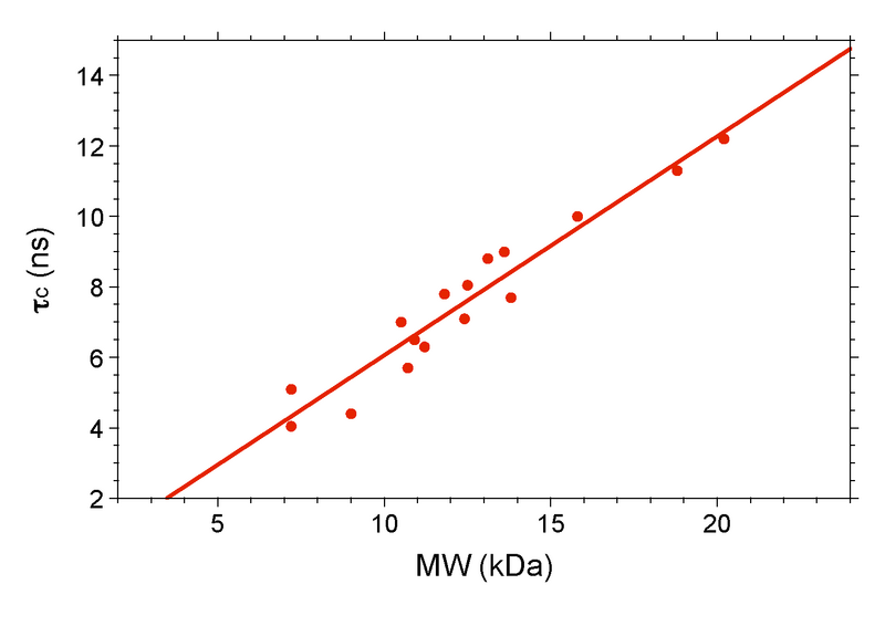
==== Figure 5: Plot of τ<sub>c</sub> vs. MW for Various NESG Monomers ==== | ==== Figure 5: Plot of τ<sub>c</sub> vs. MW for Various NESG Monomers ==== | ||
[[Image: | [[Image:T1wiki fig5.png|800x600px]]<br> | ||
== <br>'''References''' == | == <br>'''References''' == | ||
Revision as of 16:23, 11 November 2009
Introduction
The rotational correlation time of a protein in solution is the time for a protein to rotate one radian. In the limit of slow molecular motion (τc >> 0.5 ns), the correlation time of a protein is related to the ratio of the longitudinal (T1) and transverse (T2) 15N relaxation times, and nuclear frequency (νN) according to Eq. 1, which is derived from Eq. 8 in Kay et al. (Ref. 1) by considering only J(0) and J(ω) spectral densities and neglecting higher frequency terms.
In practice, global 15N T1 and T2 relaxation times for an unknown protein target can be obtained quickly (ca. 1 h) on a 1.7-mm microcyroprobe using 1D 15N-edited relaxation experiments (Ref. 2), by fitting integrated signal in the backbone amide 1H region of the spectrum as a function of delay time to an exponential decay. One then computes the correlation time using Eq. 1, and compares it to a standard curve of τc vs. protein molecular weight (MW) obtained at the same temperature on a series of known monomeric proteins of varying size. As a general rule of thumb, the τc of a monomeric protein in solution in nanoseconds is approximately 0.6 times its molecular weight in kiloDaltons. This approach is reliable up to MW ≈ 25 kDa, where accurate measurement of the diminishing 15N T2 becomes problematic.
Methods
Acquisition of 1D 15N T1 and T2 on Bruker Spectrometers
On Bruker spectrometers equipped with TopSpin 2.1 we use the hsqct1etf3gpsi3d and hsqct2etf3gpsi3d pulse sequences for the acquisition of 15N T1 and T2 spectra (Ref. 1-3). The 1D version of these experiments are acquired as pseudo 2D spectra, where the 1HN dimension is arrayed vs. delay time. We acquire 1H-detected 1D 15N relaxation spectra by using the following settings in the acquisition mode:
- set the number of acquisition points in the 15N dimension, td2 = 1
- set the number of points in the 3rd dimension equal to the number of delay times used in the experiment
- set the acquisition mode in the 3rd dimension to QF
- set NBL equal to the number of delay times used in the experiment; this is very important for the experiment to work properly
- define a vdlist (T1) or vclist (T2)
- set d1 to 3 - 5 s (T1) or 1.5 - 3 s (T2) for adequate relaxation during the experiment.
Typical vdlist and vclist files are attached.
Processing 1D 15N T1 and T2 on Bruker Spectrometers
- To process the pseudo 2D 15N relaxation date, type:
xf2
You will be prompted for a new processed data number under you experiment name.
- Next, extract the first row (into ~TEMP file) and basline correct
- Return to the processed pseudo2D apply the baseline correction using the command
bas
- Relaxation data is analyzed using the t1guide package (below) within TopSpin.
Analyzing 1D 15N T1 and T2 Data Using t1guide
For detailed information on the t1guide routine, consult the help documentation within Topspin 2.1 under Help -> Manuals -> General User Manual.
- In Topsin 2.1, launch t1guide by typing:
t1guide
- Extract the first slice of the spectrum using the Extract Slice option and expand on the amide region.
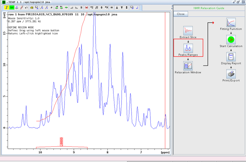
- Proceed to Peaks/Ranges and perform a manual integration (Figure 2). We typically integrate between δ ≈ 10 to 8.5 ppm. Save the integration region to disk (the diskette/A symbol in the tool bar).
Figure 1: Manual Integration of Amide Region in First Slice
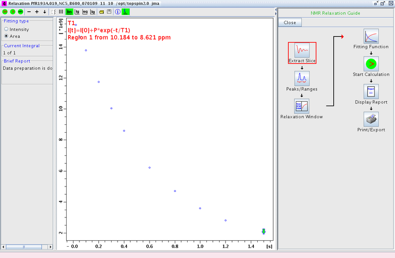
- Proceed to the Relaxation Window. A plot of integral area vs. delay time will be displayed (Figure 2). Any points that are outliers can be deleted at this point using the mouse.
Figure 2: Relaxation Window
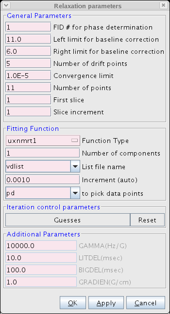
- Proceed to the Fitting Function (Figure 3). Here the user inputs various parameters including the number of points and type of function used to fit the data. We typically use the uxnmrt1 function and we prefer to use the integral area. Be sure to select the correct vdlist or vclist used in the experiment.
Figure 3: The Fitting Function
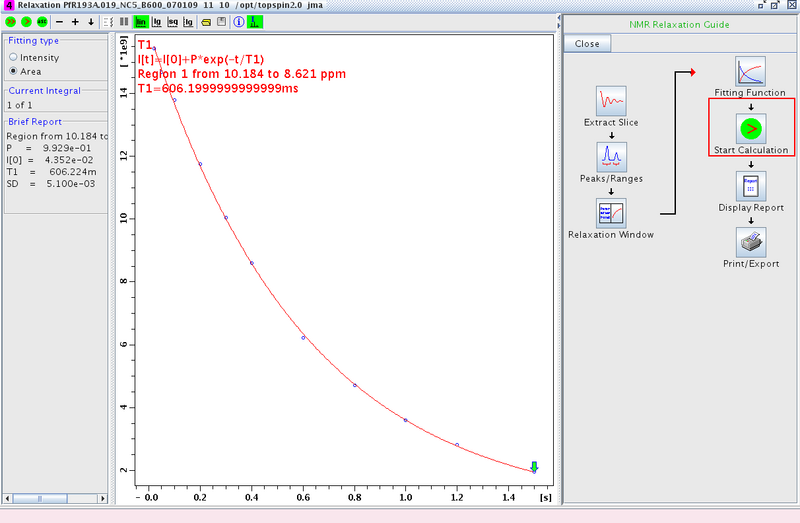
- Proceed to Start Calculation and fit the data (Figure 4)
Figure 4: Fitting the Data
- Finally, the user can also display/print the report and print the plot.
Compare the New τc to a Standard Plot
The final step in the process is to compare your τc to a standard plot of τc (ns) vs. MW (kDa) for known monomers (Figure 5). Temperature is an extremely important variable here, and it is recommended that all data be acquired at the same temperature, preferably on the same instrument. At Rutgers we have a standard curve obtained at 298 K on our Bruker 600. If your target is significantly above the curve, then it is not a monomer.
Figure 5: Plot of τc vs. MW for Various NESG Monomers
References
1. Kay, L.E., Torchia, D.A. and Bax, A. (1989) Backbone dynamics of proteins as studied by 15N inverse detected heteronuclear NMR spectroscopy: Application to staphylococcal nuclease. Biochemistry 28, 8972-8979.
2. Farrow, N.A., Muhandiram, R., Singer, A.U., Pascal, S.M., Kay, C.M., Gish, G., Shoelson, S.E., Pawson, T., Forman-Kay, J.D. and Kay, L.E. (1994) Backbone dynamics of a free and phosphopeptide-complexed Src homology 2 domain studied by 15N NMR relaxation. Biochemistry 33, 5984-6003.
3. Barbato, G., Ikura, M., Kay, L.E., Pastor, R.W. and Bax, A. (1992) Backbone dyanamics of calmodulin studied by 15N relaxation using inverse detected two-dimensional NMR spectroscopy. Biochemistry 31, 5269-5278.
-- JimAramini - 10 Nov 2009
