|
|
| (20 intermediate revisions by the same user not shown) |
| Line 1: |
Line 1: |
| ''<span style="font-size:14.0pt;mso-bidi-font-size:12.0pt">NMR Data Processing </span>''''''<span style="font-size:14.0pt">><span style="mso-spacerun: yes"> </span>RDCs</span>'''<!--StartFragment-->
| | '''NMR Data Processing > 2D HSQC-TROSY for RDCs Measurement''' <br> |
| | |
| '''2D HSQC-TROSY'''
| |
| | |
| '''<br>''' | |
|
| |
|
| ===== '''Theory/Background''' ===== | | ===== '''Theory/Background''' ===== |
|
| |
|
| <span style="mso-bidi-font-size:14.0pt;mso-bidi-font-family: Arial"> Residual Dipolar Couplings (RDCs) originate from the anisotropic
| | Residual Dipolar Couplings (RDCs) originate from the anisotropic component of the dipolar interaction, which is dependent on the angle between an internuclear vector and the magnetic field. When a molecule samples orientations uniformly, as it does in normal solution NMR, RDCs average to zero and are not observable. However, if a molecule is dissolved in a dilute liquid crystalline medium, or other orienting medium, it becomes partially aligned, and the dipolar couplings are not completely averaged to zero. This leads to a small contribution to the splitting of NMR signals. The angular dependence of these contributions can provide valuable structural information. RDCs can be used to validate protein structures, to refine structures to improve quality, and to provide constraints as a part of an initial structure determination<span style="font: 12.0px Times New Roman">.</span> RDCs can also be used to determine the rotational symmetry axis of oligomers and this information can be use to properly orient the positions of subunits within an oligomeric complex. |
| component of the dipolar interaction, which is dependent on the angle between | |
| an internuclear vector and the magnetic field. When a molecule samples | |
| orientations uniformly, as it does in normal solution NMR, RDCs average to zero | |
| and are not observable. However, if a molecule is dissolved in a dilute liquid | |
| crystalline medium, or other orienting medium, it becomes partially aligned, | |
| and the dipolar couplings are not completely averaged to zero.<span style="mso-spacerun: yes"> </span>This leads to a small contribution to the splitting of NMR signals. The angular dependence of these contributions can provide valuable structural information. <span style="mso-spacerun: yes"> </span>RDCs can be used to validate protein structures, to refine structures to improve quality, and to provide constraints as a part of an initial structure determination.<span style="mso-spacerun: yes"> </span>RDCs can also be used to determine the rotational symmetry axis of oligomers and this information can be use to properly orient the positions of subunits within an oligomeric complex.</span> | |
|
| |
|
| <br> | | <br> |
|
| |
|
| ===== '''Recent Reviews'''<br> ===== | | ===== '''Recent Reviews''' ===== |
|
| |
|
| <span style="mso-bidi-font-size: 28.0pt">Prestegard, Bougault& Kishore, ''Chemical Reviews'', '''104''',
| | Prestegard, Bougault& Kishore, ''Chemical Reviews'', '''104''', 3519-3540 (2004) |
| 3519-3540 (2004)</span> | |
|
| |
|
| <span style="mso-bidi-font-size: 28.0pt">Lipsitz& Tjandra, ''Ann. Rev. Biophys. Biomol. Struct''., '''33''',
| | Lipsitz& Tjandra, ''Ann. Rev. Biophys. Biomol. Struct''., '''33''', 387-413 (2004) |
| 387-413 (2004)</span><span style="mso-bidi-font-family:Helvetica"> </span> | |
|
| |
|
| Additional information can also be found at the following web site. | | Additional information can also be found at the following web site. |
|
| |
|
| [http://tesla.ccrc.uga.edu/courses/bionmr/lectures http://tesla.ccrc.uga.edu/courses/bionmr/lectures] | | <span style="text-decoration: underline">[http://tesla.ccrc.uga.edu/courses/bionmr/lectures http://tesla.ccrc.uga.edu/courses/bionmr/lectures]</span> |
| | |
| '''<br>'''
| |
|
| |
|
| ===== '''Brief Experimental Description'''<br> ===== | | ===== '''Brief Experimental Description''' ===== |
|
| |
|
| ''' '''HSQC-TROSY pairs provide one way of measuring RDCs.<span style="mso-spacerun: yes"> | | <span style="font: 12.0px Times New Roman">'''<span class="Apple-tab-span" style="white-space:pre"> </span>'''</span>HSQC-TROSY pairs provide one way of measuring RDCs. The procedure is applicable to proteins of small and moderate size (10-30 kDa). The acquisition time in the indirect t1 should be at least T2 of nitrogen. The measurements are easily visualized as displacements of peaks in 2D frequency domain spectra. The HSQC member of the pair gives a single peak at the center of the four peaks expected in a fully coupled HSQC experiment. The TROSY member gives only the sharpest component. The offset in either H or N direction is one half (J). Procedures for collecting this pair of experiments are described elsewhere in this Twiki (Experimental setup for HSQC-TROSY). |
| </span>The procedure is applicable to proteins of small and moderate size (10-30 kDa).<span style="mso-spacerun: yes"> </span>The acquisition time in the indirect t1 should be at least T2 of nitrogen.<span style="mso-spacerun: yes"> </span>The measurements are easily visualized as displacements of peaks in 2D frequency domain spectra. <span style="mso-spacerun: yes"> </span><span style="mso-bidi-font-size:14.0pt;mso-bidi-font-family: Arial">The HSQC member of the pair gives a single peak at the center of the
| |
| four peaks expected in a fully coupled HSQC experiment. The TROSY member gives | |
| only the sharpest component. The offset in either H or N direction is one half | |
| (J). <span style="mso-spacerun: yes"> </span>Procedures for collecting this pair of experiments are described elsewhere in this Twiki (Experimental setup for HSQC-TROSY).</span> | |
| | |
| <br>
| |
|
| |
|
| ===== '''NMR Data Processing''' ===== | | ===== '''NMR Data Processing''' ===== |
|
| |
|
| <span style="mso-bidi-font-size: 14.0pt;mso-bidi-font-family:Arial"> The data processing described below is
| | The data processing described below is specific for data collected on Varian spectrometers having the BioPack (version: 2009<span style="font: 12.0px Times New Roman">-0</span>9<span style="font: 12.0px Times New Roman">-0</span>3) sequence (gNhsqc.c) installed. Or on Bruker spectrometers having the …….. It is applied to both isotropic and aligned HSQC-TROSY pairs. |
| specific for data collected on Varian spectrometers having the BioPack | |
| (version: 2009-09-03) sequence (gNhsqc.c) installed.<span style="mso-spacerun: yes"> </span>Or on Bruker spectrometers having the …….. It is applied to both isotropic and aligned HSQC-TROSY pairs.</span> | |
|
| |
|
| '''<br>'''
| | ===== Software Information ===== |
|
| |
|
| ===== '''<span style="mso-bidi-font-size:14.0pt;mso-bidi-font-family:Arial">Required Software</span>''' =====
| | NMRPipe (download information and user manual) <br>[http://spin.niddk.nih.gov/NMRPipe/ http://spin.niddk.nih.gov/NMRPipe/] <br> <br> Brief descriptions of specific functions are accessible via nmrPipe – |
|
| |
|
| <span style="mso-bidi-font-size: 14.0pt;mso-bidi-font-family:Arial">NMRPipe</span>
| | :‘nmrPipe –help’ will list most functions. |
| | :‘nmrPipe –fn GM –help’ will give description of the GM function. |
|
| |
|
| <span style="mso-bidi-font-size: 14.0pt;mso-bidi-font-family:Arial">[http://spin.niddk.nih.gov/NMRPipe/ http://spin.niddk.nih.gov/NMRPipe/]</span> | | <br> Supported Platforms |
|
| |
|
| <br>
| | :Linux (RedHat Linux/Fedora) |
| | :Mac OS X (10.3.4 and up) |
| | :SGI Irix (6.2 and up) |
| | :Sparc Solaris (2 and up) |
| | :Windows XP Pro with Microsoft Services for UNIX (SFU 3.5) |
|
| |
|
| ===== '''<span style="mso-bidi-font-size:14.0pt;mso-bidi-font-family:Arial">Supported Platforms</span>''' ===== | | ===== '''Varian to NMRPipe Data Conversion''' ===== |
| | <pre>#!/bin/csh |
| | ##conversion of varian 2d fids into nmrPipe format for a TROSY/hsqc data set |
| | ##with array= ‘(TROSY, dm2),phase’ |
| | var2pipe -in ./fid \ |
| | -xN 2048 -yN 1024 \ |
| | -xT 1024 -yT 256 \ |
| | -xMODE Complex -yMODE Rance-Kay \ |
| | -xSW 10000.00 -ySW 2800.00 \ |
| | -xOBS 599.520 -yOBS 60.756 \ |
| | -xCAR 4.773 -yCAR 118.262 \ |
| | -xLAB HN -yLAB N \ |
| | -ndim 2 -aq2D States \ |
| | | nmrPipe -fn QMIX -ic 4 -oc 2 -cList 1 0 0 1 0 0 0 0 \ |
| | -out trosy.fid -verb -ov |
|
| |
|
| <span style="mso-bidi-font-size: 16.0pt;mso-bidi-font-family:Arial">Linux (RedHat Linux/Fedora)</span>
| | var2pipe -in ./fid \ |
| | -xN 2048 -yN 1024 \ |
| | -xT 1024 -yT 256 \ |
| | -xMODE Complex -yMODE Rance-Kay \ |
| | -xSW 10000.00 -ySW 2800.00 \ |
| | -xOBS 599.520 -yOBS 60.756 \ |
| | -xCAR 4.773 -yCAR 118.262 \ |
| | -xLAB HN -yLAB N \ |
| | -ndim 2 -aq2D States \ |
| | | nmrPipe -fn QMIX -ic 4 -oc 2 -cList 0 0 0 0 1 0 0 1 \ |
| | -out hsqc.fid -verb –ov |
| | </pre> |
| | '''Cautions:''' The usual Varian to NMRPipe macros will read in experimental parameters, but will not be able to perform data conversion since both the HSQC and TROSY spectra are collected in a interleaved manner and are stored in a single FID data file. The above script includes the QMIX function to separate fids. |
|
| |
|
| <span style="mso-bidi-font-size: 16.0pt;mso-bidi-font-family:Arial">Mac OS X (10.3.4 and up)</span>
| | ===== '''Bruker to NMRPipe Data Conversion''' ===== |
|
| |
|
| <span style="mso-bidi-font-size: 16.0pt;mso-bidi-font-family:Arial">SGI Irix <span style="mso-spacerun: yes"> </span>(6.2 and up)</span>
| | The conversion of data collected on most Bruker spectrometers can be accomplished with the following script. |
|
| |
|
| <span style="mso-bidi-font-size: 16.0pt;mso-bidi-font-family:Arial">Sparc Solaris (2 and up)</span>
| | (insert script) |
|
| |
|
| <span style="mso-bidi-font-size: 16.0pt;mso-bidi-font-family:Arial">Windows XP Pro with Microsoft Services for
| | ===== '''Fourier Transformation of Converted HSQC and TROSY spectra''' ===== |
| UNIX (SFU 3.5).</span>
| |
|
| |
|
| <br> | | The following script contains some data specific parameters including phasing parameters and convolution functions that will need to be optimized for each specific set. |
| | <pre>#!/bin/csh |
| | #This script is to process one of the TROSY/ |
| | | nmrPipe -in hsqc.fid \ |
| | | nmrPipe -fn SOL \ |
| | | nmrPipe -fn SP -off 0.5 -end 0.99 -pow 2 -c 0.5 \ |
| | | nmrPipe -fn ZF -auto \ |
| | | nmrPipe -fn FT \ |
| | | nmrPipe -fn PS -p0 -61.6 -p1 -4.6 -di \ |
| | | nmrPipe -fn EXT -x1 6.00ppm -xn 11.50ppm -verb 2 -sw \ |
| | | nmrPipe -fn TP \ |
| | | nmrPipe -fn LP -x1 1 -xn 256 -pred 256 -after -verb \ |
| | | nmrPipe -fn SP -off 0.5 -end 0.99 -pow 2 -c 1.0 \ |
| | | nmrPipe -fn ZF -auto \ |
| | | nmrPipe -fn FT \ |
| | | nmrPipe -fn PS -p0 -91.8 -p1 7.0 -di \ |
| | | nmrPipe -fn TP \ |
| | | nmrPipe -fn EXT -y1 100.00ppm -yn 138.00ppm -sw \ |
| | | nmrPipe -out hsqc.ft2 -verb 2 -ov |
| | </pre> |
|
| |
|
| ===== '''Varian to NMRPipe data conversion''' ===== | | ===== '''RDC Assignment and Calculation''' ===== |
|
| |
|
| <span style="font-size:8.0pt;mso-bidi-font-size:11.0pt; font-family:Courier;mso-bidi-font-family:Courier;color:#7D4700">#!/bin/csh</span>
| | '''General Concepts''' |
|
| |
|
| <span style="font-size:8.0pt;mso-bidi-font-size:11.0pt; font-family:Courier;mso-bidi-font-family:Courier;color:#7D4700"># conversion of | | Transfer all assignments (or cross peak labels) from a reference isotropic HSQC spectrum to TROSY and HSQC spectra obtained under both isotropic and aligned conditions. The positions of cross-peaks in the aligned HSQC spectrum usually change little with addition of an alignment medium; if they do change, there is often a constant offset for all peaks due to changes in the lock resonance<span style="font: 12.0px Times New Roman">.</span> Hence<span style="font: 12.0px Times New Roman">,</span> transferring assignments is usually straightforward. Corresponding peaks for TROSY assignments are diagonally displaced (down and to the right) by 38-58 Hz. The isotropic coupling (J) is calculated from the difference in Hz between the <sup>15</sup>N dimension of isotropic HSQC and TROSY spectra (the offset is one half (J), so the final value needs to be multiply by 2). Similarly, the aligned coupling (J+D) is calculated from differences in peak positions for the aligned HSQC and TROSY spectra. The Hz values of the corresponding peaks can be subtracted using a spreadsheet or script to calculate the RDC values. |
| varian 2d fids into nmrPipe format for a TROSY/hsqc data set</span>
| |
|
| |
|
| <span style="font-size:8.0pt;mso-bidi-font-size:11.0pt; font-family:Courier;mso-bidi-font-family:Courier;color:#7D4700"># with array= ‘(TROSY,
| | The peak picking and assignment process can be done using any graphical NMR assignment program of user’s choice. NMRViewJ has a special feature that would match and transfer assignment from one spectrum to another. For this tutorial, we have included a Tcl/TK script for obtaining RDCs using NMRDraw and NMRWish; the process is broken down into five steps. |
| dm2),phase’</span>
| |
|
| |
|
| <span style="font-size:8.0pt;mso-bidi-font-size:11.0pt; font-family:Courier;mso-bidi-font-family:Courier;color:#7D4700">var2pipe -in | | <br> |
| ./fid \</span>
| |
|
| |
|
| <span style="font-size:8.0pt;mso-bidi-font-size:11.0pt; font-family:Courier;mso-bidi-font-family:Courier;color:#7D4700"><span style="mso-spacerun: yes"> </span>-xN<span style="mso-spacerun: yes">
| | ===== '''RDC Assignment and Calculation Scripts''' ===== |
| </span>2048<span style="mso-spacerun: yes"> </span>-yN<span style="mso-spacerun: yes"> </span>1024<span style="mso-spacerun: yes"> </span>\</span>
| |
|
| |
|
| <span style="font-size:8.0pt;mso-bidi-font-size:11.0pt; font-family:Courier;mso-bidi-font-family:Courier;color:#7D4700"><span style="mso-spacerun: yes"> </span></span><span lang="FR" style="font-size:8.0pt;mso-bidi-font-size:11.0pt;font-family:Courier; mso-bidi-font-family:Courier;color:#7D4700;mso-ansi-language:FR">-xT<span style="mso-spacerun: yes">
| | '''Step 1: step1_hsqc_ass.tcl''' <br> |
| </span>1024<span style="mso-spacerun: yes"> </span>-yT<span style="mso-spacerun: yes"> </span>256<span style="mso-spacerun: yes"> </span>\</span>
| |
|
| |
|
| <span lang="FR" style="font-size:8.0pt;mso-bidi-font-size: 11.0pt;font-family:Courier;mso-bidi-font-family:Courier;color:#7D4700; mso-ansi-language:FR"><span style="mso-spacerun: yes">
| | '''Function:''' Automatically pick peaks in NMRDraw for the isotropic HSQC spectrum and save the peak list as hsqc.tab to be use as reference peak list. This script cuts out vast amounts of non-essential data that are stored in the hsqc.tab file after initial peak picking, leaving only the labels and, HN and N ppm values. |
| </span>-xMODE<span style="mso-spacerun: yes">
| |
| </span>Complex<span style="mso-spacerun: yes">
| |
| </span>-yMODE<span style="mso-spacerun: yes"> </span>Rance-Kay<span style="mso-spacerun: yes"> </span>\</span>
| |
|
| |
|
| <span lang="FR" style="font-size:8.0pt;mso-bidi-font-size: 11.0pt;font-family:Courier;mso-bidi-font-family:Courier;color:#7D4700; mso-ansi-language:FR"><span style="mso-spacerun: yes"> </span></span><span style="font-size:8.0pt;mso-bidi-font-size:11.0pt;font-family:Courier; mso-bidi-font-family:Courier;color:#7D4700">-xSW<span style="mso-spacerun: yes"> </span>10000.00<span style="mso-spacerun: yes"> </span>-ySW<span style="mso-spacerun: yes"> </span>2800.00<span style="mso-spacerun: yes"> </span>\</span> | | <br> |
|
| |
|
| <span style="font-size:8.0pt;mso-bidi-font-size:11.0pt; font-family:Courier;mso-bidi-font-family:Courier;color:#7D4700"><span style="mso-spacerun: yes"> </span>-xOBS<span style="mso-spacerun: yes"> </span>599.520<span style="mso-spacerun: yes"> </span>-yOBS<span style="mso-spacerun: yes"> </span>60.756<span style="mso-spacerun: yes"> </span>\</span>
| | '''Execution:''' Executing this script does not require code modification. The only requirement is that you add the output and input script names in the execution line of a LINUX operating system<span style="font: 12.0px Times New Roman">.</span> |
|
| |
|
| <span style="font-size:8.0pt;mso-bidi-font-size:11.0pt; font-family:Courier;mso-bidi-font-family:Courier;color:#7D4700"><span style="mso-spacerun: yes"> </span>-xCAR<span style="mso-spacerun: yes"> </span>4.773<span style="mso-spacerun: yes"> </span>-yCAR<span style="mso-spacerun: yes"> </span>118.262<span style="mso-spacerun: yes"> </span>\</span> | | <br> |
|
| |
|
| <span style="font-size:8.0pt;mso-bidi-font-size:11.0pt; font-family:Courier;mso-bidi-font-family:Courier;color:#7D4700"><span style="mso-spacerun: yes"> </span>-xLAB<span style="mso-spacerun: yes">
| | '''Command: ''' |
| </span>HN<span style="mso-spacerun: yes"> </span>-yLAB<span style="mso-spacerun: yes">
| | <pre>./step1_hsqc_ass.tcl hsqc_ass.tab hsqc.tab</pre> |
| </span>N<span style="mso-spacerun: yes"> </span>\</span>
| | Where “hsqc_ass.tab” is the output file and “hsqc.tab” is the input file to this script. |
|
| |
|
| <span style="font-size:8.0pt;mso-bidi-font-size:11.0pt; font-family:Courier;mso-bidi-font-family:Courier;color:#7D4700"><span style="mso-spacerun: yes"> </span>-ndim<span style="mso-spacerun: yes"> | | <br> |
| </span>2<span style="mso-spacerun: yes"> </span>-aq2D<span style="mso-spacerun: yes"> </span>States<span style="mso-spacerun: yes"> </span>\</span>
| |
|
| |
|
| <span style="font-size:8.0pt;mso-bidi-font-size:11.0pt; font-family:Courier;mso-bidi-font-family:Courier;color:#7D4700"><span style="mso-spacerun: yes"> </span>| nmrPipe -fn QMIX -ic 4 -oc 2 -cList 1 0 0 1 0 0 0 0<span style="mso-spacerun: yes"> </span>\</span>
| | Download: [[Media:Step1_hsqc_ass.tcl|Step1_hsqc_ass.tcl]] |
|
| |
|
| <span style="font-size:8.0pt;mso-bidi-font-size:11.0pt; font-family:Courier;mso-bidi-font-family:Courier;color:#7D4700"><span style="mso-spacerun: yes"> </span></span><span lang="NO-BOK" style="font-size:8.0pt;mso-bidi-font-size:11.0pt;font-family:Courier; mso-bidi-font-family:Courier;color:#7D4700;mso-ansi-language:NO-BOK">-out | | <br> |
| trosy.fid -verb -ov</span>
| |
|
| |
|
| | '''Step 2: i-hsqctrosy_step2.tcl''' |
|
| |
|
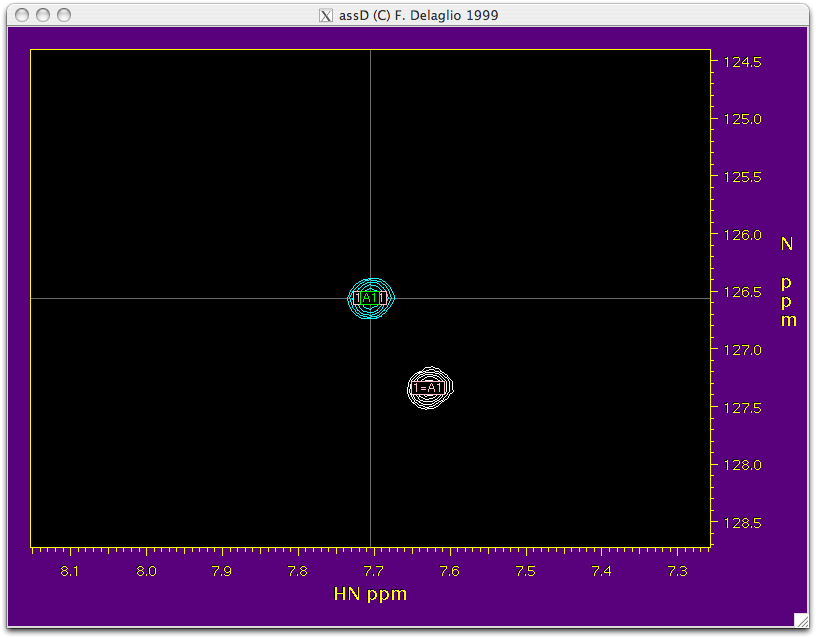
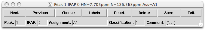
| | '''Function:''' This script takes the HSQC and TROSY peak tables that you created while peak picking and combines them into a single table. It also transfers the assignment from the isotropic HSQC to HSQC aligned, TROSY isotropic and TROSY aligned spectra. On execution, it opens “NMRWish” which can further help in transferring the assignment peak by peak from HSQC to HSQC-TROSY. All the blue peaks in the NMRWish display belong to the HSQC spectrum and the white peaks belong to the TROSYspectrum. The peak under consideration is on the crosswire of the NMRWish window. A navigation bar will also appear along with the NMRWish display to allow user to visually inspect the assignment of each peak and make corrections if necessary. |
|
| |
|
| <span lang="NO-BOK" style="font-size:8.0pt;mso-bidi-font-size: 11.0pt;font-family:Courier;mso-bidi-font-family:Courier;color:#7D4700; mso-ansi-language:NO-BOK">var2pipe -in ./fid \</span>
| | [[Image:Step2-spectrum.png|Step2-spectrum.png]] [[Image:Step2-navi.png|Step2-navi.png]] <br> |
|
| |
|
| <span lang="NO-BOK" style="font-size:8.0pt;mso-bidi-font-size: 11.0pt;font-family:Courier;mso-bidi-font-family:Courier;color:#7D4700; mso-ansi-language:NO-BOK"><span style="mso-spacerun: yes"> </span></span><span style="font-size:8.0pt;mso-bidi-font-size:11.0pt;font-family:Courier; mso-bidi-font-family:Courier;color:#7D4700">-xN<span style="mso-spacerun: yes">
| | '''Execution:''' Executing this script requires editing the script file itself and changing a few values. Make sure that '''assName '''(from step 1)''', tabName1'''(peak table for HSQC)''', tabName2''' (peak table for TROSY)''', and outName '''(output file name) have the correct input table names. You must also enter the height (contour level) at which you picked the peaks for hsqc in the '''hi1 '''field and the height at which you picked peaks for trosy in the '''hi2''' field. Also make sure that the correct names for the .ft2 spectrum are specified in the script. |
| </span>2048<span style="mso-spacerun: yes"> </span>-yN<span style="mso-spacerun: yes"> </span>1024<span style="mso-spacerun: yes"> </span>\<o:p></o:p></span>
| |
|
| |
|
| <span style="font-size:8.0pt;mso-bidi-font-size:11.0pt; font-family:Courier;mso-bidi-font-family:Courier;color:#7D4700"><span style="mso-spacerun: yes"> </span></span><span lang="FR" style="font-size:8.0pt;mso-bidi-font-size:11.0pt;font-family:Courier; mso-bidi-font-family:Courier;color:#7D4700;mso-ansi-language:FR">-xT<span style="mso-spacerun: yes">
| | |
| </span>1024<span style="mso-spacerun: yes"> </span>-yT<span style="mso-spacerun: yes"> </span>256<span style="mso-spacerun: yes"> </span>\<o:p></o:p></span>
| |
|
| |
|
| <span lang="FR" style="font-size:8.0pt;mso-bidi-font-size: 11.0pt;font-family:Courier;mso-bidi-font-family:Courier;color:#7D4700; mso-ansi-language:FR"><span style="mso-spacerun: yes">
| | '''Command: ''' |
| </span>-xMODE<span style="mso-spacerun: yes"> | | <pre>./i-hsqctrosy_step2.tcl</pre> |
| </span>Complex<span style="mso-spacerun: yes"> | | <br> |
| </span>-yMODE<span style="mso-spacerun: yes"> </span>Rance-Kay<span style="mso-spacerun: yes"> </span>\<o:p></o:p></span> | |
|
| |
|
| <span lang="FR" style="font-size:8.0pt;mso-bidi-font-size: 11.0pt;font-family:Courier;mso-bidi-font-family:Courier;color:#7D4700; mso-ansi-language:FR"><span style="mso-spacerun: yes"> </span></span><span style="font-size:8.0pt;mso-bidi-font-size:11.0pt;font-family:Courier; mso-bidi-font-family:Courier;color:#7D4700">-xSW<span style="mso-spacerun: yes"> </span>10000.00<span style="mso-spacerun: yes"> </span>-ySW<span style="mso-spacerun: yes"> </span>2800.00<span style="mso-spacerun: yes"> </span>\<o:p></o:p></span>
| | Download: [[Media:I-hsqctrosy_step2.tcl|I-hsqctrosy_step2.tcl]] |
|
| |
|
| <span style="font-size:8.0pt;mso-bidi-font-size:11.0pt; font-family:Courier;mso-bidi-font-family:Courier;color:#7D4700"><span style="mso-spacerun: yes"> </span>-xOBS<span style="mso-spacerun: yes"> </span>599.520<span style="mso-spacerun: yes"> </span>-yOBS<span style="mso-spacerun: yes"> </span>60.756<span style="mso-spacerun: yes"> </span>\<o:p></o:p></span> | | <br> |
|
| |
|
| <span style="font-size:8.0pt;mso-bidi-font-size:11.0pt; font-family:Courier;mso-bidi-font-family:Courier;color:#7D4700"><span style="mso-spacerun: yes"> </span>-xCAR<span style="mso-spacerun: yes"> </span>4.773<span style="mso-spacerun: yes"> </span>-yCAR<span style="mso-spacerun: yes"> </span>118.262<span style="mso-spacerun: yes"> </span>\<o:p></o:p></span>
| | '''Step 3: i-hsqctrosy_step3.tcl''' |
|
| |
|
| <span style="font-size:8.0pt;mso-bidi-font-size:11.0pt; font-family:Courier;mso-bidi-font-family:Courier;color:#7D4700"><span style="mso-spacerun: yes"> </span>-xLAB<span style="mso-spacerun: yes">
| | '''Function:''' This script calculates the coupling values for the protein. |
| </span>HN<span style="mso-spacerun: yes"> </span>-yLAB<span style="mso-spacerun: yes">
| |
| </span>N<span style="mso-spacerun: yes"> </span>\<o:p></o:p></span>
| |
|
| |
|
| <span style="font-size:8.0pt;mso-bidi-font-size:11.0pt; font-family:Courier;mso-bidi-font-family:Courier;color:#7D4700"><span style="mso-spacerun: yes"> </span>-ndim<span style="mso-spacerun: yes"> | | <br> |
| </span>2<span style="mso-spacerun: yes"> </span>-aq2D<span style="mso-spacerun: yes"> </span>States<span style="mso-spacerun: yes"> </span>\<o:p></o:p></span>
| |
|
| |
|
| <span style="font-size:8.0pt;mso-bidi-font-size:11.0pt; font-family:Courier;mso-bidi-font-family:Courier;color:#7D4700"><span style="mso-spacerun: yes"> </span>| nmrPipe -fn QMIX -ic 4 -oc 2 -cList 0 0 0 0 1 0 0 1<span style="mso-spacerun: yes"> </span>\<o:p></o:p></span>
| | '''Execution:''' Execution of this script requires that you open up the script and change the '''inName''' to the output of step 2. It also requires that you once again input the '''hi1''' and '''hi2''' values just like you did in step 2. |
|
| |
|
| <span style="font-size:8.0pt;mso-bidi-font-size:11.0pt; font-family:Courier;mso-bidi-font-family:Courier;color:#7D4700"><span style="mso-spacerun: yes"> </span><span style="mso-spacerun: yes"> </span>-out hsqc.fid -verb –ov<o:p></o:p></span> | | <br> |
|
| |
|
| '''<br>''' | | '''Command:''' |
| | <pre>./i-hsqctrosy_step3.tcl</pre> |
| | <br> |
|
| |
|
| '''<span style="mso-bidi-font-size:11.0pt;mso-bidi-font-family:Courier">Cautions:</span>'''<span style="mso-bidi-font-size:11.0pt;mso-bidi-font-family:Courier"> The usual
| | Download: [[Media:I-hsqctrosy_step3.tcl|I-hsqctrosy_step3.tcl]] |
| Varian to NMRPipe macros will read in experimental parameters, but will not be
| |
| able to perform data conversion since both the HSQC and TROSY spectra are
| |
| collected in a interleaved manner and are stored in a single FID data
| |
| file.<span style="mso-spacerun: yes"> </span>The above script includes the QMIX function to separate fids.</span>
| |
|
| |
|
| <br> | | <br> |
|
| |
|
| ===== '''Bruker to NMRPipe data conversion''' =====
| | '''Step 4: i-hsqctrosy_step4.tcl''' |
|
| |
|
| <span style="mso-bidi-font-size:11.0pt;mso-bidi-font-family: Courier"><o:p> </o:p></span>
| | '''Function:''' This script cleans up the output from the previous script (step 3) and outputs the necessary information (chemical shift of H and N in ppm and coupling values) into a new text file. |
|
| |
|
| <span style="mso-bidi-font-size:11.0pt;mso-bidi-font-family: Courier"><span style="mso-tab-count:1"> </span>The conversion of data collected on most Bruker spectrometers can be accomplished with the following script.<span style="mso-spacerun: yes"> </span>The same precautions pertain?<o:p></o:p></span> | | <br> |
|
| |
|
| <span style="mso-bidi-font-size:11.0pt;mso-bidi-font-family: Courier">(insert script)<o:p></o:p></span>
| | '''Execution:''' Execution of this script requires that you change a single variable in the script. Make sure that you set the '''outName''' variable to the proper media type (gel, peg, iso, etc…). |
|
| |
|
| <span style="mso-bidi-font-size:11.0pt;mso-bidi-font-family: Courier"><o:p> </o:p></span> | | <br> |
|
| |
|
| '''<span style="mso-bidi-font-size:11.0pt;mso-bidi-font-family:Courier">2.6<span style="mso-tab-count:1"> </span>Fourier transformation of converted HSQC and TROSY spectra<o:p></o:p></span>''' | | '''Command:''' |
| | <pre>./i-hsqctrosy_step4.tcl</pre> |
| | <br> |
|
| |
|
| '''<span style="font-size:8.0pt;mso-bidi-font-size:11.0pt;font-family:Courier; mso-bidi-font-family:Courier;color:#7D4700"><o:p> </o:p></span>'''
| | Download: [[Media:I-hsqctrosy_step4.tcl|I-hsqctrosy_step4.tcl]] |
|
| |
|
| '''<span style="font-size:8.0pt;mso-bidi-font-size:11.0pt;font-family:Courier; mso-bidi-font-family:Courier;color:#7D4700"><span style="mso-tab-count:1"> </span></span>'''<span style="mso-bidi-font-family:Courier;color:#7D4700">The following script
| | <br> |
| contains some data specific parameters including phasing parameters and
| |
| convolution functions that will need to be optimized for each specific set.<o:p></o:p></span>
| |
|
| |
|
| <span style="mso-bidi-font-family:Courier;color:#7D4700"><o:p> </o:p></span>
| | '''Step 5: i-hsqctrosy_step5.tcl''' |
|
| |
|
| '''<span style="font-size:8.0pt;mso-bidi-font-size:11.0pt;font-family:Courier; mso-bidi-font-family:Courier;color:#7D4700">#!/bin/csh<o:p></o:p></span>''' | | '''Function:''' This script calculates the rdc values for the protein. |
|
| |
|
| <span style="font-size:8.0pt;mso-bidi-font-size:11.0pt; font-family:Courier;mso-bidi-font-family:Courier;color:#7D4700"># This script | | <br> |
| is to process one of the TROSY/<o:p></o:p></span>
| |
|
| |
|
| <span style="font-size:8.0pt;mso-bidi-font-size:11.0pt; font-family:Courier;mso-bidi-font-family:Courier;color:#7D4700">| nmrPipe<span style="mso-spacerun: yes"> </span>-in hsqc.fid<span style="mso-spacerun: yes">
| | '''Execution:''' We recommend that a new folder be created in the protein directory titled '''rdc_name?''' to organize and retain all of the files required to run this script. Copy or Move all of the required files into the '''rdc '''folder; these include: '''hsqc_ass.tab''' file and all of the '''*_j.tab''' files generated from isotropic data and each medium. Make sure that the '''assName, isoName, '''and '''othName '''We recommend the '''outName''' field to have the naming convention '''protein.name_rdc_media.tab''' (ex. rnr77_rdc_gel). |
| </span>\<o:p></o:p></span>
| |
|
| |
|
| <span style="font-size:8.0pt;mso-bidi-font-size:11.0pt; font-family:Courier;mso-bidi-font-family:Courier;color:#7D4700">| nmrPipe -fn
| | ''' ''' |
| SOL<span style="mso-spacerun: yes"> </span>\<o:p></o:p></span>
| |
|
| |
|
| <span style="font-size:8.0pt;mso-bidi-font-size:11.0pt; font-family:Courier;mso-bidi-font-family:Courier;color:#7D4700">| nmrPipe<span style="mso-spacerun: yes"> </span>-fn SP -off 0.5 -end 0.99 -pow 2 -c 0.5<span style="mso-spacerun: yes"> </span>\<o:p></o:p></span>
| | '''Command:''' |
| | | <pre>./i-hsqctrosy_step5.tcl</pre> |
| <span style="font-size:8.0pt;mso-bidi-font-size:11.0pt; font-family:Courier;mso-bidi-font-family:Courier;color:#7D4700">| nmrPipe<span style="mso-spacerun: yes"> </span>-fn ZF -auto<span style="mso-spacerun: yes">
| | <br> |
| </span>\<o:p></o:p></span>
| |
| | |
| <span style="font-size:8.0pt;mso-bidi-font-size:11.0pt; font-family:Courier;mso-bidi-font-family:Courier;color:#7D4700">| nmrPipe<span style="mso-spacerun: yes"> </span>-fn FT<span style="mso-spacerun: yes">
| |
| </span><span style="mso-spacerun: yes"> </span>\<o:p></o:p></span>
| |
| | |
| <span style="font-size:8.0pt;mso-bidi-font-size:11.0pt; font-family:Courier;mso-bidi-font-family:Courier;color:#7D4700">| nmrPipe -fn
| |
| PS -p0 -61.6 -p1 -4.6<span style="mso-spacerun: yes"> </span>-di<span style="mso-spacerun: yes"> </span>\<o:p></o:p></span>
| |
| | |
| <span style="font-size:8.0pt;mso-bidi-font-size:11.0pt; font-family:Courier;mso-bidi-font-family:Courier;color:#7D4700">| nmrPipe<span style="mso-spacerun: yes"> </span>-fn EXT -x1 6.00ppm -xn 11.50ppm -verb 2 -sw<span style="mso-spacerun: yes"> </span>\<o:p></o:p></span>
| |
| | |
| <span style="font-size:8.0pt;mso-bidi-font-size:11.0pt; font-family:Courier;mso-bidi-font-family:Courier;color:#7D4700">| nmrPipe -fn
| |
| TP<span style="mso-spacerun: yes">
| |
| </span>\<o:p></o:p></span>
| |
| | |
| <span style="font-size:8.0pt;mso-bidi-font-size:11.0pt; font-family:Courier;mso-bidi-font-family:Courier;color:#7D4700">| nmrPipe -fn
| |
| LP -x1 1 -xn 256 -pred 256 -after -verb<span style="mso-spacerun: yes"> </span>\<o:p></o:p></span>
| |
| | |
| <span style="font-size:8.0pt;mso-bidi-font-size:11.0pt; font-family:Courier;mso-bidi-font-family:Courier;color:#7D4700">| nmrPipe -fn
| |
| SP -off 0.5 -end 0.99 -pow 2 -c 1.0<span style="mso-spacerun: yes">
| |
| </span>\<o:p></o:p></span>
| |
| | |
| <span style="font-size:8.0pt;mso-bidi-font-size:11.0pt; font-family:Courier;mso-bidi-font-family:Courier;color:#7D4700">| nmrPipe -fn
| |
| ZF -auto<span style="mso-spacerun: yes"> </span>\<o:p></o:p></span>
| |
| | |
| <span style="font-size:8.0pt;mso-bidi-font-size:11.0pt; font-family:Courier;mso-bidi-font-family:Courier;color:#7D4700">| nmrPipe -fn
| |
| FT<span style="mso-spacerun: yes">
| |
| </span>\<o:p></o:p></span>
| |
| | |
| <span style="font-size:8.0pt;mso-bidi-font-size:11.0pt; font-family:Courier;mso-bidi-font-family:Courier;color:#7D4700">| nmrPipe -fn
| |
| PS -p0 -91.8 -p1 7.0<span style="mso-spacerun: yes">
| |
| </span>-di<span style="mso-spacerun: yes"> </span>\<o:p></o:p></span>
| |
| | |
| <span style="font-size:8.0pt;mso-bidi-font-size:11.0pt; font-family:Courier;mso-bidi-font-family:Courier;color:#7D4700">| nmrPipe -fn
| |
| TP<span style="mso-spacerun: yes">
| |
| </span>\<o:p></o:p></span>
| |
| | |
| <span style="font-size:8.0pt;mso-bidi-font-size:11.0pt; font-family:Courier;mso-bidi-font-family:Courier;color:#7D4700">| nmrPipe -fn
| |
| EXT -y1 100.00ppm -yn<span style="mso-spacerun: yes">
| |
| </span>138.00ppm -sw \<o:p></o:p></span>
| |
| | |
| <span style="font-size:8.0pt;mso-bidi-font-size:11.0pt; font-family:Courier;mso-bidi-font-family:Courier;color:#7D4700">| nmrPipe -out
| |
| hsqc.ft2 -verb 2 -ov</span><span style="font-size:8.0pt;mso-bidi-font-size: 11.0pt;mso-bidi-font-family:Courier"><o:p></o:p></span>
| |
| | |
| <span style="font-size:8.0pt;mso-bidi-font-size:11.0pt; mso-bidi-font-family:Courier"><o:p> </o:p></span>
| |
| | |
| <span style="mso-bidi-font-size:11.0pt;mso-bidi-font-family: Courier"><o:p> </o:p></span>
| |
| | |
| '''<span style="mso-bidi-font-size:14.0pt;mso-bidi-font-family:Arial">3.0<span style="mso-tab-count:1"> </span>RDC Assignment and Calculation<o:p></o:p></span>'''
| |
| | |
| '''<span style="mso-bidi-font-size:14.0pt;mso-bidi-font-family:Arial"><o:p> </o:p></span>'''
| |
| | |
| '''<span style="mso-bidi-font-size:14.0pt;mso-bidi-font-family:Arial">3.1<span style="mso-tab-count:1"> </span>General Concepts</span>'''<span style="mso-bidi-font-size:14.0pt;mso-bidi-font-family: Arial"> <o:p></o:p></span>
| |
| | |
| <span style="mso-bidi-font-size:14.0pt;mso-bidi-font-family: Arial">Transfer all assignments (or cross peak labels) from a reference isotropic
| |
| HSQC spectrum to TROSY and HSQC spectra obtained under both isotropic and
| |
| aligned conditions. <span style="mso-spacerun: yes"> </span>The positions of<span style="mso-spacerun: yes"> </span>cross-peaks in the aligned HSQC spectrum usually change little with addition of an alignment medium; if they do change, there is often a constant offset for all peaks due to changes in the lock resonance.<span style="mso-spacerun: yes"> </span>Hence, transferring assignments is usually straightforward. Corresponding peaks for TROSY assignments are diagonally displaced (down and to the right) by 38-58 Hz.<span style="mso-spacerun: yes"> </span>The isotropic coupling (J) is calculated from the difference in Hz<span style="mso-spacerun: yes">
| |
| </span>between the <sup>15</sup>N dimension of isotropic HSQC and TROSY spectra (the offset is one half (J), so the final value needs to be multiply by 2).<span style="mso-spacerun: yes"> </span>Similarly, the aligned coupling (J+D) is calculated from differences in peak positions for the aligned HSQC and TROSY spectra.<span style="mso-spacerun: yes"> </span>The Hz values of the corresponding peaks can be subtracted using a spreadsheet or script to calculate the RDC values.<o:p></o:p></span>
| |
| | |
| <span style="mso-bidi-font-size:14.0pt;mso-bidi-font-family: Arial">The peak picking and assignment process can be done using any graphical
| |
| NMR assignment program of user’s choice.<span style="mso-spacerun: yes">
| |
| </span>NMRViewJ has a special feature that would match and transfer assignment from one spectrum to another.<span style="mso-spacerun: yes">
| |
| </span>For this tutorial, we have included a Tcl/TK script for obtaining RDCs using NMRDraw and NMRWish; the process is broken down into five steps.<o:p></o:p></span>
| |
| | |
| <span style="mso-bidi-font-size:14.0pt;mso-bidi-font-family: Arial"><o:p> </o:p></span>
| |
| | |
| '''<span style="mso-bidi-font-size:14.0pt;mso-bidi-font-family:Arial">3.2<span style="mso-tab-count:1"> </span>RDC Scripts<o:p></o:p></span>'''
| |
| | |
| '''<span style="mso-bidi-font-size:14.0pt;mso-bidi-font-family:Arial"><o:p> </o:p></span>'''
| |
| | |
| '''<span style="mso-bidi-font-size:14.0pt;mso-bidi-font-family:Arial">3.2.1<span style="mso-tab-count:1"> </span>Step 1: step1_hsqc_ass.tcl<o:p></o:p></span>'''
| |
| | |
| '''<o:p> </o:p>'''
| |
| | |
| '''Function:''' <span style="mso-bidi-font-size:14.0pt;mso-bidi-font-family:Arial">Automatically pick
| |
| peaks in NMRDraw for the isotropic HSQC spectrum and save the peak list as
| |
| hsqc.tab to be use as reference peak list.</span> <span style="mso-spacerun: yes"> </span>This script cuts out vast amounts of<span style="mso-spacerun: yes"> </span>non-essential data that are stored in the hsqc.tab file after initial peak picking, leaving only the labels and, HN and N ppm values.'''<span style="mso-bidi-font-size: 14.0pt;mso-bidi-font-family:Arial"><o:p></o:p></span>'''
| |
| | |
| <o:p> </o:p>
| |
| | |
| '''Execution:''' Executing this script does not require code modification. The only requirement is that you add the output and input script names in the execution line of a LINUX operating system.<o:p></o:p>
| |
| | |
| <o:p> </o:p>
| |
| | |
| '''Command: <o:p></o:p>''' | |
| | |
| ./step1_hsqc_ass.tcl hsqc_ass.tab hsqc.tab<o:p></o:p>
| |
| | |
| Where “hsqc_ass.tab” is the output file and “hsqc.tab” is the input file to this script.<o:p></o:p>
| |
| | |
| <o:p> </o:p>
| |
| | |
| Download: step1_hsqc_ass.tcl <span style="mso-spacerun: yes"> </span><span style="font-size:11.0pt;mso-bidi-font-size:14.0pt; mso-bidi-font-family:Arial"><o:p></o:p></span>
| |
| | |
| <span style="font-size:11.0pt;mso-bidi-font-size:14.0pt; mso-bidi-font-family:Arial"><o:p> </o:p></span> | |
| | |
| '''3.2.2<span style="mso-tab-count:1"> </span>Step 2: i-hsqctrosy_step2.tcl<o:p></o:p>'''
| |
| | |
| <o:p> </o:p>
| |
| | |
| '''Function:''' This script takes the HSQC and TROSY peak tables that you created while peak picking and combines them into a single table. It also transfers the assignment from the isotropic HSQC to HSQC aligned, TROSY isotropic and TROSY aligned spectra. On execution, it opens “NMRWish” which can further help in transferring the assignment peak by peak from HSQC to HSQC-TROSY. All the blue peaks in the NMRWish display belong to the HSQC spectrum and the white peaks belong to the TROSYspectrum. The peak under consideration is on the crosswire of the NMRWish window.<span style="mso-spacerun: yes"> </span>A navigation bar will also appear along with the NMRWish display to allow user to visually inspect the assignment of each peak and make corrections if necessary.<o:p></o:p>
| |
| | |
| <o:p> </o:p>
| |
| | |
| '''Execution:''' Executing this script requires editing the script file itself and changing a few values. Make sure that '''assName '''(from step 1)''', tabName1'''(peak table for HSQC)''', tabName2''' (peak table for TROSY)''', and outName '''(output file name) have the correct input table names. You must also enter the height (contour level) at which you picked the peaks for hsqc in the '''hi1 '''field and the height at which you picked peaks for trosy in the '''hi2''' field. Also make sure that the correct names for the .ft2 spectrum are specified in the script. <o:p></o:p>
| |
| | |
| <span style="mso-spacerun: yes"> </span><o:p></o:p> | |
| | |
| '''Command: <o:p></o:p>'''
| |
| | |
| ./i-hsqctrosy_step2.tcl<o:p></o:p>
| |
| | |
| <o:p> </o:p>
| |
| | |
| Download: i-hsqctrosy_step2.tcl<o:p></o:p>
| |
| | |
| <o:p> </o:p>
| |
| | |
| '''3.2.3<span style="mso-tab-count:1"> </span>Step 3: i-hsqctrosy_step3.tcl'''<o:p></o:p>
| |
| | |
| <o:p> </o:p>
| |
| | |
| '''Function:''' This script calculates the coupling values for the protein.<o:p></o:p>
| |
| | |
| <o:p> </o:p>
| |
| | |
| '''Execution:''' Execution of this script requires that you open up the script and change the '''inName''' to the output of step 2. It also requires that you once again input the '''hi1''' and '''hi2''' values just like you did in step 2.<o:p></o:p>
| |
| | |
| <o:p> </o:p>
| |
| | |
| '''Command:<o:p></o:p>'''
| |
| | |
| ./i-hsqctrosy_step3.tcl<o:p></o:p>
| |
| | |
| <span style="mso-bidi-font-size:14.0pt;mso-bidi-font-family: Arial"><o:p> </o:p></span>
| |
| | |
| <span style="mso-bidi-font-size:14.0pt;mso-bidi-font-family: Arial">Download: i-hsqctrosy_step3.tcl<o:p></o:p></span>
| |
| | |
| <span style="mso-bidi-font-size:14.0pt;mso-bidi-font-family: Arial"><o:p> </o:p></span>
| |
| | |
| '''3.2.4<span style="mso-tab-count:1"> </span>Step 4: i-hsqctrosy_step4.tcl'''<o:p></o:p>
| |
| | |
| <o:p> </o:p>
| |
| | |
| '''Function:''' This script cleans up the output from the previous script (step 3) and outputs the necessary information (chemical shift of H and N in ppm and coupling values) into a new text file. <o:p></o:p>
| |
| | |
| <o:p> </o:p>
| |
| | |
| '''Execution:''' Execution of this script requires that you change a single variable in the script. Make sure that you set the '''outName''' variable to the proper media type (gel, peg, iso, etc…). <o:p></o:p>
| |
| | |
| <o:p> </o:p>
| |
| | |
| '''Command:<o:p></o:p>'''
| |
| | |
| ./i-hsqctrosy_step4.tcl<o:p></o:p>
| |
| | |
| <span style="mso-bidi-font-size:14.0pt;mso-bidi-font-family: Arial"><o:p> </o:p></span>
| |
| | |
| <span style="mso-bidi-font-size:14.0pt;mso-bidi-font-family: Arial">Download: i-hsqctrosy_step4.tcl<o:p></o:p></span>
| |
| | |
| <span style="mso-bidi-font-size:14.0pt;mso-bidi-font-family: Arial"><o:p> </o:p></span>
| |
| | |
| '''3.2.5<span style="mso-tab-count:1"> </span>Step 5: i-hsqctrosy_step5.tcl'''<o:p></o:p>
| |
| | |
| <o:p> </o:p>
| |
| | |
| '''Function:''' This script calculates the rdc values for the protein.<o:p></o:p>
| |
| | |
| <o:p> </o:p>
| |
| | |
| '''Execution:''' We recommend that a new folder be created in the protein directory titled '''rdc_name?''' to organize and retain all of the files required to run this script. Copy or Move all of the required files into the '''rdc '''folder; these include: '''hsqc_ass.tab''' file and all of the '''*_j.tab''' files generated from isotropic data and each medium. Make sure that the '''assName, isoName, '''and '''othName '''We recommend the '''outName''' field to have the naming convention '''protein.name_rdc_media.tab''' (ex. rnr77_rdc_gel).<o:p></o:p>
| |
| | |
| '''<span style="mso-spacerun: yes"> </span><o:p></o:p>'''
| |
| | |
| '''Command:<o:p></o:p>'''
| |
| | |
| ./i-hsqctrosy_step5.tcl<o:p></o:p>
| |
| | |
| <o:p> </o:p>
| |
|
| |
|
| <span style="mso-bidi-font-size:14.0pt;mso-bidi-font-family: Arial">Download: i-hsqctrosy_step5.tcl<o:p></o:p></span> <!--EndFragment-->
| | Download: [[Media:I-hsqctrosy_step5.tcl|I-hsqctrosy_step5.tcl]] |
| | <br> |
| | <br> |
| | <br> |
| | Updated by Hsiau-Wei Lee, 2011 |
NMR Data Processing > 2D HSQC-TROSY for RDCs Measurement
Theory/Background
Residual Dipolar Couplings (RDCs) originate from the anisotropic component of the dipolar interaction, which is dependent on the angle between an internuclear vector and the magnetic field. When a molecule samples orientations uniformly, as it does in normal solution NMR, RDCs average to zero and are not observable. However, if a molecule is dissolved in a dilute liquid crystalline medium, or other orienting medium, it becomes partially aligned, and the dipolar couplings are not completely averaged to zero. This leads to a small contribution to the splitting of NMR signals. The angular dependence of these contributions can provide valuable structural information. RDCs can be used to validate protein structures, to refine structures to improve quality, and to provide constraints as a part of an initial structure determination. RDCs can also be used to determine the rotational symmetry axis of oligomers and this information can be use to properly orient the positions of subunits within an oligomeric complex.
Recent Reviews
Prestegard, Bougault& Kishore, Chemical Reviews, 104, 3519-3540 (2004)
Lipsitz& Tjandra, Ann. Rev. Biophys. Biomol. Struct., 33, 387-413 (2004)
Additional information can also be found at the following web site.
http://tesla.ccrc.uga.edu/courses/bionmr/lectures
Brief Experimental Description
HSQC-TROSY pairs provide one way of measuring RDCs. The procedure is applicable to proteins of small and moderate size (10-30 kDa). The acquisition time in the indirect t1 should be at least T2 of nitrogen. The measurements are easily visualized as displacements of peaks in 2D frequency domain spectra. The HSQC member of the pair gives a single peak at the center of the four peaks expected in a fully coupled HSQC experiment. The TROSY member gives only the sharpest component. The offset in either H or N direction is one half (J). Procedures for collecting this pair of experiments are described elsewhere in this Twiki (Experimental setup for HSQC-TROSY).
NMR Data Processing
The data processing described below is specific for data collected on Varian spectrometers having the BioPack (version: 2009-09-03) sequence (gNhsqc.c) installed. Or on Bruker spectrometers having the …….. It is applied to both isotropic and aligned HSQC-TROSY pairs.
Software Information
NMRPipe (download information and user manual)
http://spin.niddk.nih.gov/NMRPipe/
Brief descriptions of specific functions are accessible via nmrPipe –
- ‘nmrPipe –help’ will list most functions.
- ‘nmrPipe –fn GM –help’ will give description of the GM function.
Supported Platforms
- Linux (RedHat Linux/Fedora)
- Mac OS X (10.3.4 and up)
- SGI Irix (6.2 and up)
- Sparc Solaris (2 and up)
- Windows XP Pro with Microsoft Services for UNIX (SFU 3.5)
Varian to NMRPipe Data Conversion
#!/bin/csh
##conversion of varian 2d fids into nmrPipe format for a TROSY/hsqc data set
##with array= ‘(TROSY, dm2),phase’
var2pipe -in ./fid \
   -xN           2048    -yN      1024   \
   -xT           1024    -yT      256   \
   -xMODE     Complex    -yMODE   Rance-Kay  \
   -xSW       10000.00   -ySW      2800.00  \
   -xOBS      599.520    -yOBS      60.756   \
   -xCAR         4.773    -yCAR    118.262   \
   -xLAB           HN    -yLAB         N   \
   -ndim            2    -aq2D    States   \
   | nmrPipe -fn QMIX -ic 4 -oc 2 -cList 1 0 0 1 0 0 0 0   \
   -out trosy.fid -verb -ov

var2pipe -in ./fid \
  -xN           2048    -yN      1024   \
   -xT           1024    -yT      256   \
   -xMODE     Complex    -yMODE   Rance-Kay  \
   -xSW       10000.00   -ySW     2800.00  \
   -xOBS      599.520    -yOBS      60.756   \
   -xCAR         4.773    -yCAR    118.262   \
   -xLAB           HN    -yLAB         N   \
   -ndim            2    -aq2D    States   \
   | nmrPipe -fn QMIX -ic 4 -oc 2 -cList 0 0 0 0 1 0 0 1   \
   -out hsqc.fid -verb –ov
Cautions: The usual Varian to NMRPipe macros will read in experimental parameters, but will not be able to perform data conversion since both the HSQC and TROSY spectra are collected in a interleaved manner and are stored in a single FID data file. The above script includes the QMIX function to separate fids.
Bruker to NMRPipe Data Conversion
The conversion of data collected on most Bruker spectrometers can be accomplished with the following script.
(insert script)
Fourier Transformation of Converted HSQC and TROSY spectra
The following script contains some data specific parameters including phasing parameters and convolution functions that will need to be optimized for each specific set.
#!/bin/csh
#This script is to process one of the TROSY/
| nmrPipe  -in hsqc.fid              \
| nmrPipe -fn SOL   \
| nmrPipe  -fn SP -off 0.5 -end 0.99 -pow 2 -c 0.5  \
| nmrPipe  -fn ZF -auto                    \
| nmrPipe  -fn FT                     \
| nmrPipe -fn PS -p0 -61.6 -p1 -4.6  -di    \
| nmrPipe  -fn EXT -x1 6.00ppm -xn 11.50ppm -verb 2 -sw  \
| nmrPipe -fn TP                      \
| nmrPipe -fn LP -x1 1 -xn 256 -pred 256 -after -verb   \
| nmrPipe -fn SP -off 0.5 -end 0.99 -pow 2 -c 1.0  \
| nmrPipe -fn ZF -auto           \
| nmrPipe -fn FT                   \
| nmrPipe -fn PS -p0 -91.8 -p1 7.0   -di     \
| nmrPipe -fn TP        \
| nmrPipe -fn EXT -y1 100.00ppm -yn    138.00ppm -sw \
| nmrPipe -out hsqc.ft2 -verb 2 -ov
RDC Assignment and Calculation
General Concepts
Transfer all assignments (or cross peak labels) from a reference isotropic HSQC spectrum to TROSY and HSQC spectra obtained under both isotropic and aligned conditions. The positions of cross-peaks in the aligned HSQC spectrum usually change little with addition of an alignment medium; if they do change, there is often a constant offset for all peaks due to changes in the lock resonance. Hence, transferring assignments is usually straightforward. Corresponding peaks for TROSY assignments are diagonally displaced (down and to the right) by 38-58 Hz. The isotropic coupling (J) is calculated from the difference in Hz between the 15N dimension of isotropic HSQC and TROSY spectra (the offset is one half (J), so the final value needs to be multiply by 2). Similarly, the aligned coupling (J+D) is calculated from differences in peak positions for the aligned HSQC and TROSY spectra. The Hz values of the corresponding peaks can be subtracted using a spreadsheet or script to calculate the RDC values.
The peak picking and assignment process can be done using any graphical NMR assignment program of user’s choice. NMRViewJ has a special feature that would match and transfer assignment from one spectrum to another. For this tutorial, we have included a Tcl/TK script for obtaining RDCs using NMRDraw and NMRWish; the process is broken down into five steps.
RDC Assignment and Calculation Scripts
Step 1: step1_hsqc_ass.tcl
Function: Automatically pick peaks in NMRDraw for the isotropic HSQC spectrum and save the peak list as hsqc.tab to be use as reference peak list. This script cuts out vast amounts of non-essential data that are stored in the hsqc.tab file after initial peak picking, leaving only the labels and, HN and N ppm values.
Execution: Executing this script does not require code modification. The only requirement is that you add the output and input script names in the execution line of a LINUX operating system.
Command:
./step1_hsqc_ass.tcl hsqc_ass.tab hsqc.tab
Where “hsqc_ass.tab” is the output file and “hsqc.tab” is the input file to this script.
Download: Step1_hsqc_ass.tcl
Step 2: i-hsqctrosy_step2.tcl
Function: This script takes the HSQC and TROSY peak tables that you created while peak picking and combines them into a single table. It also transfers the assignment from the isotropic HSQC to HSQC aligned, TROSY isotropic and TROSY aligned spectra. On execution, it opens “NMRWish” which can further help in transferring the assignment peak by peak from HSQC to HSQC-TROSY. All the blue peaks in the NMRWish display belong to the HSQC spectrum and the white peaks belong to the TROSYspectrum. The peak under consideration is on the crosswire of the NMRWish window. A navigation bar will also appear along with the NMRWish display to allow user to visually inspect the assignment of each peak and make corrections if necessary.
Execution: Executing this script requires editing the script file itself and changing a few values. Make sure that assName (from step 1), tabName1(peak table for HSQC), tabName2 (peak table for TROSY), and outName (output file name) have the correct input table names. You must also enter the height (contour level) at which you picked the peaks for hsqc in the hi1 field and the height at which you picked peaks for trosy in the hi2 field. Also make sure that the correct names for the .ft2 spectrum are specified in the script.
Command:
./i-hsqctrosy_step2.tcl
Download: I-hsqctrosy_step2.tcl
Step 3: i-hsqctrosy_step3.tcl
Function: This script calculates the coupling values for the protein.
Execution: Execution of this script requires that you open up the script and change the inName to the output of step 2. It also requires that you once again input the hi1 and hi2 values just like you did in step 2.
Command:
./i-hsqctrosy_step3.tcl
Download: I-hsqctrosy_step3.tcl
Step 4: i-hsqctrosy_step4.tcl
Function: This script cleans up the output from the previous script (step 3) and outputs the necessary information (chemical shift of H and N in ppm and coupling values) into a new text file.
Execution: Execution of this script requires that you change a single variable in the script. Make sure that you set the outName variable to the proper media type (gel, peg, iso, etc…).
Command:
./i-hsqctrosy_step4.tcl
Download: I-hsqctrosy_step4.tcl
Step 5: i-hsqctrosy_step5.tcl
Function: This script calculates the rdc values for the protein.
Execution: We recommend that a new folder be created in the protein directory titled rdc_name? to organize and retain all of the files required to run this script. Copy or Move all of the required files into the rdc folder; these include: hsqc_ass.tab file and all of the *_j.tab files generated from isotropic data and each medium. Make sure that the assName, isoName, and othName We recommend the outName field to have the naming convention protein.name_rdc_media.tab (ex. rnr77_rdc_gel).
Command:
./i-hsqctrosy_step5.tcl
Download: I-hsqctrosy_step5.tcl
Updated by Hsiau-Wei Lee, 2011

